- Author: Turhan Can Kargın and Kamil Gültekin
- Topic: Vision-Based Control Course Project
The project we prepared for the Vision-based Control lecture, which is one of the Poznan University of Technology Automatic Control and Robotics graduate courses. In this project, you will find couple of projects that can be helpful to learn Image Processing, Computer Vision, Deep Neural Network, Convolutional Neural Network topics and OpenCV, Tensorflow, Keras, YOLO Frameworks.
- Summary
- Introduction
- Image Classifiaction
- Object Detection
- Object Recognition
- Object Tracking
- Project Lists
- Object Detection with Specific Color
- Motion Detection and Tracking with OpenCV
- Face and Eye Detection with OpenCV and Haar Feature based Cascade Classifiers
- MNIST Image Classification with Deep Neural Network
- MNIST Image Classification with Convolutional Neural Network
- Real Time Digit Classification
- Real Time Object Recognition with SSD
- Future Work
- References
In this repository, the details of image processing and computer vision are discussed. In addition, convolutional neural networks, which are frequently used in deep learning-based computer vision applications, are explained. In addition to these, seven basic level projects were exhibited in this repository to provide reinforcement on the topics discussed.
Mankind continues the data processing process, which started by drawing animal figures on the cave walls, with "chips" that are too small to be seen by the human eye. Although this development spanned a long period of approximately 4000 years, the real development took place in the last 50 years. It was impossible for human beings to even predict this technology, which has entered every aspect of our lives today and has become a routine of our lives. For example; A manager of IBM, one of the important companies in the computer industry, said, "No matter how small a computer gets, it cannot be smaller than a room." The fact that one of the leading names in the industry is so wrong explains how fast computer technology has developed. In this development process, human beings, who are no longer content with their own intelligence, are also trying to give intelligence to machines; Now the goal is to produce machines that are more intelligent, capable of sampling human behavior, perceiving and interpreting images, characterizing sounds and, as a result, making decisions.
Although the foundations of image formation go back centuries, intensive studies on machine imaging systems started with the introduction of special equipment. With the developments in technology, the use of imaging systems; production lines, medicine, weapons systems, criminology and security spanned many areas.
Today, systems with automatic movement capability include a large share of the technological development process. In the progress of robot systems, researchers have to use sensors similar to the ones that humans have, opening up to the outside world, and develop perception principles in similar ways in order to produce systems that can make faster, more dynamic and more accurate decisions. In addition, this way of working should be close to the working speed of humanoid functions and should be produced in real time.
With the transfer of the image to the computer environment, there have been significant developments in the speed and capacity ratios of image processing devices. With each advancing year, digital image processors that allow obtaining higher resolution and pixelated images have begun to be developed. High resolution and pixel ratio have revealed high data capacity and significant developments have been experienced in recording environments. Many manufacturers have tried to impose their own recording standard, and along with this, image processing devices using very different recording media have been introduced to the market.
Many factors in the field of image processing point to continuous improvement. One of the main reasons is the falling prices of necessary computer equipment. The processing units required are getting cheaper every year. A second factor is the increase in hardware options required for digitizing and displaying images. The indications are that the prices of essential computer hardware will continue to fall. Many new technologies are developing in a way that allows the expansion of studies in this field. Microprocessors, CCDs used for digitization, new memory technologies and high resolution image systems etc. Another acceleration in development is due to the continuous continuation of new applications. The uses of digital imaging in advertising, industrial, medical and scientific research continue to grow. Significant reduction in hardware costs and the ability to make important applications show that image processing techniques will play an important role in the future.
In addition, Computer Vision-based Robot systems is one of the fields that researchers have studied intensively. This issue, which is in parallel with the development of especially high-tech security solutions, industrial applications that require complex perceptions and defense technologies, has become the main study target for today's practitioners.
This repository has discussed in detail the concepts of image processing and computer vision, which have recently entered our lives with the developing technology, together with the applications.
This repository consists of eight main sections. The first one is the introductory part, which deals with computer vision, image processing and their difference, and also talks about neural networks and their algorithms and frameworks. The second, third, fourth and fifth sectionss are considered as image classification, object detection, recognition and tracking. There is a project list section at sixth section that describing the projects done. Finally, you can find future works and references as last two sections.
Image processing is a method that can be identified with different techniques in order to obtain useful information according to the relevant need through the images transferred to the digital media. The image processing method is used to process certain recorded images and modify existing images and graphics to alienate or improve them. For example, it is possible to see the quality declines when scanning photos or documents and transferring them to digital media. This is where the image processing method comes into play during the quality declines. We use image processing method to minimize the degraded image quality and visual distortions. Another example is the maps that we can access via Google Earth. Satellite images are enhanced by image processing techniques. In this way, people are presented with higher quality images. Image processing, which can be used in this and many other places, is among the rapidly developing technologies. It is also one of the main research areas of disciplines such as engineering and computer science [1].
 Image processing is basically studied in three steps.
- Transferring the image with the necessary tools
- Analyzing the image and processing it in the desired direction
- Receiving the results of the data report and output that are analyzed and processed
In addition to the image processing steps, two types of methods are used for image processing. The first is analog image processing and the other is digital image processing. There are a number of basic steps that data must go through for digital and analog image processing. These steps are as follows:
- Preprocessing
- Development and viewing
- Information extraction
After these steps, results can be obtained from the relevant data according to the needs.
Image processing has purposes such as visualization, making partially visible objects visible, image enhancement, removing spots, noise removal, high resolution capture in the image, pattern, and shape recognition.
Some techniques which are used in digital image processing include:
- Anisotropic diffusion
- Hidden Markov models
- Image editing
- Image restoration
- Independent component analysis
- Linear filtering
- Neural networks
- Partial differential equations
- Pixelation
- Point feature matching
- Principal components analysis
- Self-organizing maps
- Wavelets
Human perception of the outside world is formed by perceiving and analyzing images, which is one of the most important perception channels, and interpreting them. All techniques aiming to create visual perception and understanding in humans on the computer fall into the field of computer vision and cognitive learning. Scientists working in the field of computer vision have played the biggest role in the advancement of artificial intelligence, which is the most mentioned deep learning sub-field today.
Computer vision aims to make sense of all kinds of two-dimensional, three-dimensional or higher-dimensional visual digital data, especially with smart algorithms. In solving these problems, the field of computer vision uses the development and implementation of both mathematical and computational theory-based techniques such as geometry, linear algebra, probability and statistics theory, differential equations, graph theory, and in recent years, especially machine learning and deep learning. In addition to standard camera images, medical images, satellite images, and computer modeling of three-dimensional objects and scenes are of interest to computer vision.
Visual data detection and interpretation constitute the most important algorithm steps in many applications, from autonomous systems such as autonomous vehicles, robots, drones, to security and biometric verification areas. The outputs obtained are fed as inputs to the decision support systems in the next step, completing the artificial intelligence systems [2].
Computer vision has emerged as a critical research topic, with commercial applications based on computer vision approaches accounting for a significant share of the market. Over the years, the accuracy and speed with which images acquired by cameras are processed and identified has improved. Deep learning, being the most well-known lad in town, is playing a vital role as a computer vision technology.
Is deep learning the only way to accomplish computer vision? No, no, no! A few years ago, deep learning made its debut in the field of computer vision. Image processing algorithms and approaches were the mainstays of computer vision at the time. The main task of computer vision was to extract the image's features. When doing a computer vision task, the initial stage was to detect color, edges, corners, and objects. These features are human-engineered, and the extracted features, as well as the methodologies employed for feature extraction, have a direct impact on the model's accuracy and reliability. In the traditional vision scope, the algorithms like SIFT (Scale-Invariant Feature Transform), SURF (Speeded-Up Robust Features), BRIEF (Binary Robust Independent Elementary Features) plays the major role of extracting the features from the raw image.
The difficulty with this approach of feature extraction in image classification is that you have to choose which features to look for in each given image. When the number of classes of the classification goes high or the image clarity goes down it’s really hard to cope up with traditional computer vision algorithms.
In the field of computer vision, deep learning, which is a subset of machine learning, has shown considerable performance and accuracy gains. In a popular ImageNet computer vision competition in 2012, a neural network with over 60 million parameters greatly outperformed previous state-of-the-art algorithms to picture recognition, arguably one of the most influential studies in bringing deep learning to computer vision.

The boom started with the convolutional neural networks and the modified architectures of ConvNets. By now it is said that some convNet architectures are so close to 100% accuracy of image classification challenges, sometimes beating the human eye!
The main difference in deep learning approach of computer vision is the concept of end-to-end learning. There’s no longer need of defining the features and do feature engineering. The neural do that for you. It can simply put in this way. Though deep neural networks has its major drawbacks like, need of having huge amount of training data and need of large computation power, the field of computer vision has already conquered by this amazing tool already!
Computer vision and image processing are both attractive fields of computer science.
In computer vision, computers or machines are programmed to extract high-level information from digital images or videos as input, with the goal of automating operations that the human visual system can perform. It employs a variety of techniques, including Image Processing.
Image processing is the science of enhancing photographs by adjusting a variety of parameters and attributes. As a result, Image Processing is considered a subset of Computer Vision. In this case, transformations are made to an input image, and the resulting image is returned. Sharpening, smoothing, stretching, and other changes are examples of these transformations.
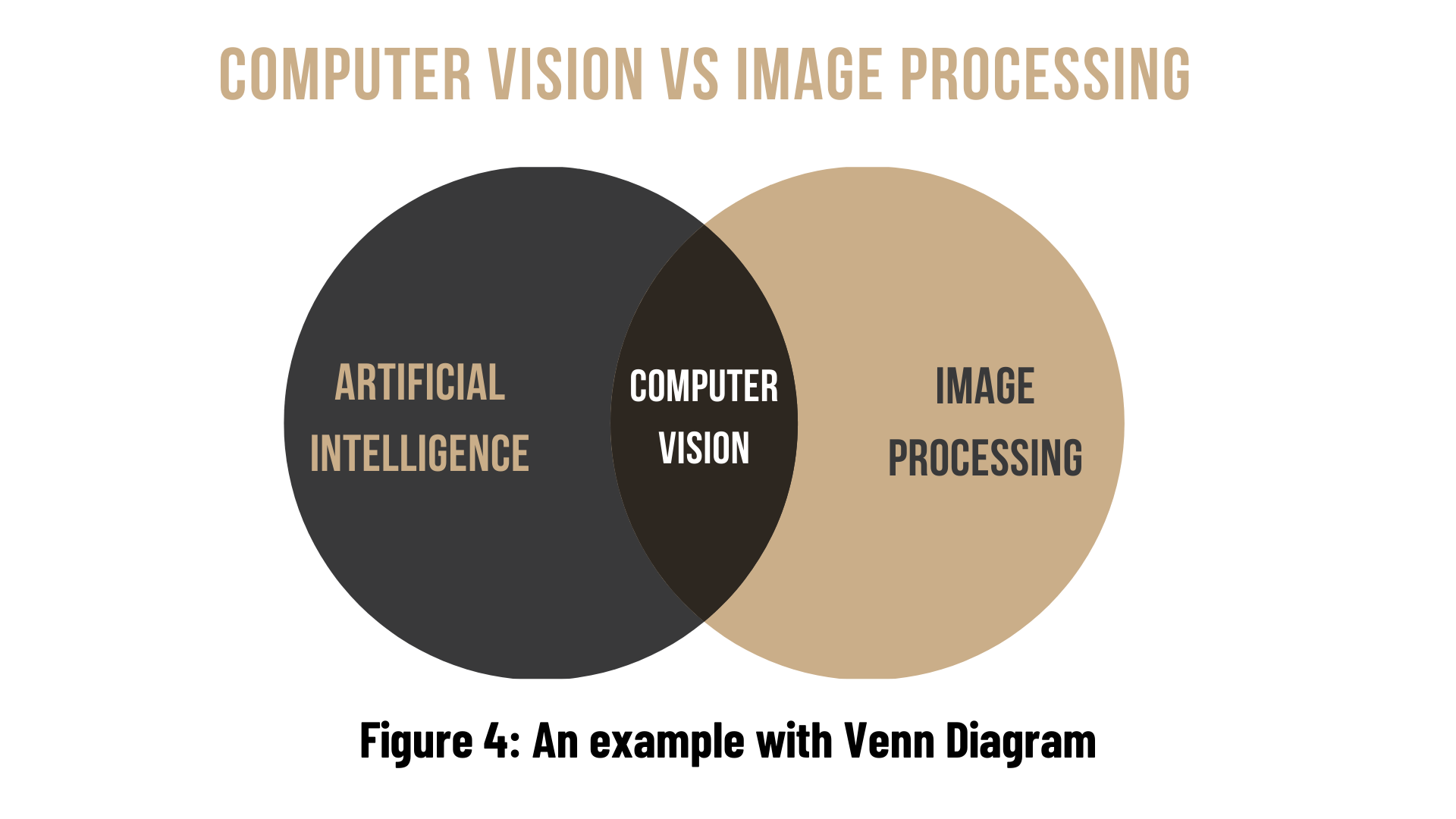
Both of the fields is working with visuals, i.e., images and videos. In fact, although it is not very accurate, we can say that if you use artificial intelligence algorithms and image processing methods in a project, that project is probably turning into a Computer Vision project. So Computer Vision is an intersection of Artificial Intelligence and Image Processing that usually aims to simulate intelligent human abilities.
| Image Processing | Computer Vision |
|---|---|
| Image processing is mainly focused on processing the raw input images to enhance them or preparing them to do other tasks | Computer vision is focused on extracting information from the input images or videos to have a proper understanding of them to predict the visual input like human brain. |
| Image processing uses methods like Anisotropic diffusion, Hidden Markov models, Independent component analysis, Different Filtering etc. | Image processing is one of the methods that is used for computer vision along with other Machine learning techniques, CNN etc. |
| Image Processing is a subset of Computer Vision. | Computer Vision is a superset of Image Processing. |
| Examples of some Image Processing applications are- Rescaling image (Digital Zoom), Correcting illumination, Changing tones etc. | Examples of some Computer Vision applications are- Object detection, Face detection, Hand writing recognition etc. |
Deep neural networks are a field of research in which researchers show great interest under the science of artificial intelligence. It covers studies on learning computers. In this section, firstly, a general introduction to artificial intelligence will be given, then deep neural networks will be examined, and then the most widely used deep learning frameworks will be examined.
Computers and computer systems have become an indispensable part of life in the contemporary world. Many devices, from mobile phones to refrigerators in kitchens, work with computer systems. It has become commonplace to use computers in almost every field, from the business world to public affairs, from environmental and health organizations to military systems. When the development of technology is followed, it is seen that computers, which were previously developed only for electronic data transfer and performing complex calculations, gain qualifications that can filter and summarize large amounts of data over time and make comments about events using existing information. Today, computers can both make decisions about events and learn the relationships between events.
Problems that cannot be formulated mathematically and cannot be solved can be solved by computers using heuristic methods. Studies that equip computers with these features and enable them to develop these abilities are known as "artificial intelligence" studies. Artificial intelligence, in its simplest definition, is the general name of systems that try to imitate a certain part of human intelligence. From this point of view, when it comes to artificial intelligence, we should not think of systems that can completely imitate human intelligence or that have this purpose.
Artificial intelligence can show itself in many different areas: Systems that predict what we write in our daily life, the search engine that allows us to search for an image on Google, Youtube's video recommendation system, and Instagram, which is very curious about how it once worked, is frequently ranked by those who see the story. are the examples we encountered.
Deep learning, a sub-branch of Artificial Intelligence, is simply the name we give to training multi-layer artificial neural networks (Multi Layer Artificial Neural Networks) with an algorithm called "backpropagation". Even these two concepts are broad concepts that can be explained by books on their own. Artificial neural networks (ANNs), which are used in deep learning, are computer software that perform basic functions such as learning, remembering, and generating new data from the data it collects by imitating the learning path of the human brain. Artificial neural networks, inspired by the human brain, emerged as a result of the mathematical modeling of the learning process.
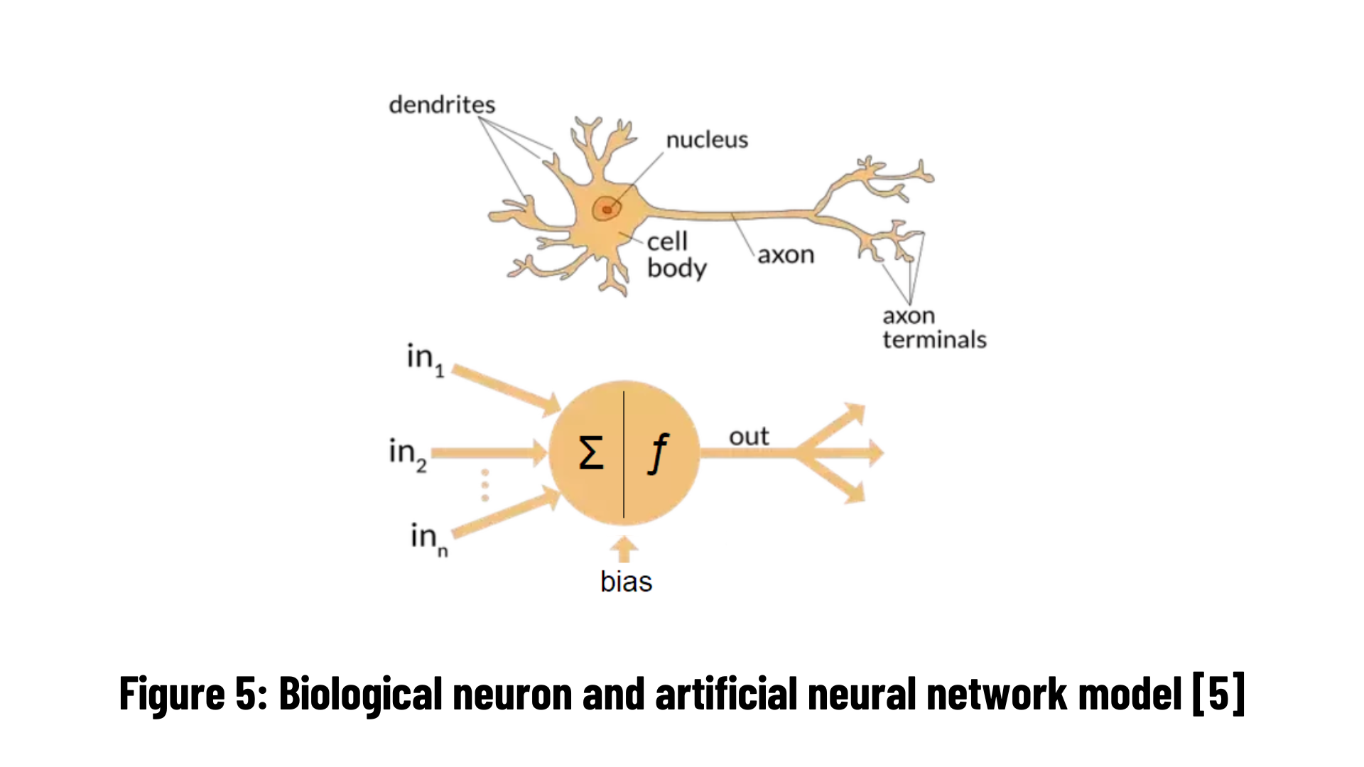
Biological neuron and artificial neural network simulations are given in Figure 5. Biological Nervous system elements and their equivalents in the artificial nervous system are given in table below. Here, the biological nervous system is divided into parts and each element is given an equivalent in the artificial neural network system.
| Biological Neuron System | Artificial NeuronSystem |
|---|---|
| Neuron | Processor Element |
| Dendrite | Aggregation Function |
| Cell Body | Transfer Function |
| Axons | Artificial Neuron Output |
| Synapses | Weights |
As seen in below gift, dog and cat data enters the network. The data processed in the middle layers is sent from there to the output layer. In short, this process is the conversion of incoming information to the output using the weight values of the network. In order for the network to produce the correct outputs for the inputs, the weights must have the correct values.

If you want to get more detailed information about artificial neural networks, you can click on this link. Let's take a look at the most widely used deep learning frameworks.
PyTorch is an optimized tensor library for deep learning using GPUs and CPUs.
 PyTorch was published by Facebook in 2017 as a Python-based and open-source machine learning library connected to Torch. There is also a C/C++ interface. It offers a faster experience by using graphics processing units. This makes it superior and preferable to other libraries. It is preferred because it is more compatible with the structure we call Pythonic, that is, with various libraries in Python (numpy…). It is also easy and simple to understand. It does not act on a single Back-End. It offers different models for GPUs. What we call Back-End is the name given to the server in the background and the work of developing the base software. It uses dynamic computational graphics. The advantage of dynamic computational graphs lies in their ability to adapt to varying amounts in the input data.
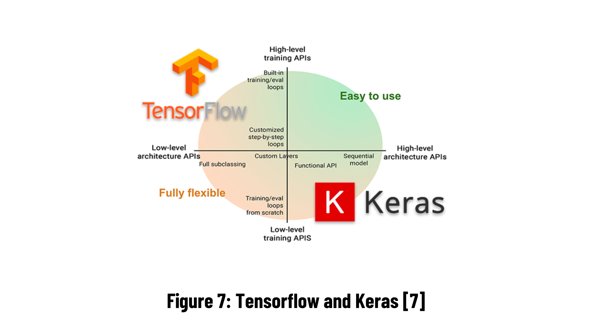
Keras is a deep learning library for Python used in machine learning. The biggest advantage of Keras is that it can run on libraries such as TensorFlow, Theano. It is ideal for beginners as it is easily and quickly accessible. It can run on CPU and GPU. You can choose whatever you want to save time. It supports convolutional neural networks (CNN) and iterative neural networks (RNN). There are quite a lot of resources on the internet because large companies have so many users, so when faced with a problem, the solution becomes simpler. TensorFlow is likewise an open source deep learning library. It can be used on CPU and GPU. Although it is based on Python, it supports multiple languages (C++, Java, C#, Javascript, R…).
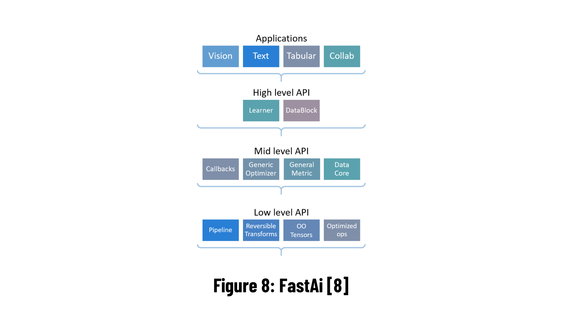
fastai is a deep learning library which provides practitioners with high-level components that can quickly and easily provide state-of-the-art results in standard deep learning domains, and provides researchers with low-level components that can be mixed and matched to build new approaches. It aims to do both things without substantial compromises in ease of use, flexibility, or performance. This is possible thanks to a carefully layered architecture, which expresses common underlying patterns of many deep learning and data processing techniques in terms of decoupled abstractions. These abstractions can be expressed concisely and clearly by leveraging the dynamism of the underlying Python language and the flexibility of the PyTorch library. fastai includes:
- A new type dispatch system for Python along with a semantic type hierarchy for tensors
- A GPU-optimized computer vision library which can be extended in pure Python
- An optimizer which refactors out the common functionality of modern optimizers into two basic pieces, allowing optimization algorithms to be implemented in 4–5 lines of code
- A novel 2-way callback system that can access any part of the data, model, or optimizer and change it at any point during training
- A new data block API
- And much more...
fastai is organized around two main design goals: to be approachable and rapidly productive, while also being deeply hackable and configurable. It is built on top of a hierarchy of lower-level APIs which provide composable building blocks. This way, a user wanting to rewrite part of the high-level API or add particular behavior to suit their needs does not have to learn how to use the lowest level.
Convolutional neural networks take pictures or videos as input due to their structure. Of course, when taking pictures, they must be translated into the relevant format. For example, if we are giving a picture to a convolutional neural network, we need to export it in matrix format.
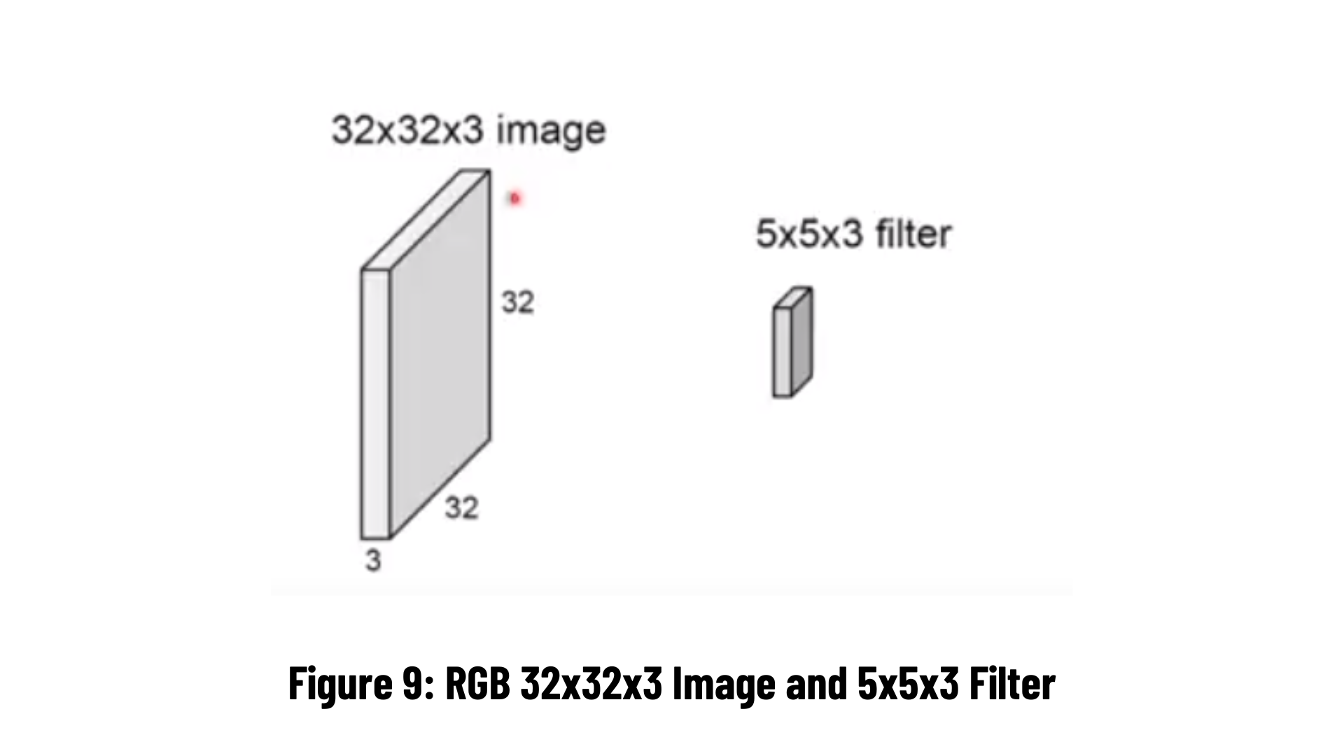 We see 32x32 and 5x5 matrices in Figure 9. The 3 next to them indicate the RGB value, that is, it is colored. (It is 1 in black and white) Thanks to the filter we apply to the matrix, data is obtained from the picture by comparing certain features on the picture. Let's now go deeper in CNN.
The symmetry of the filter to be applied to the two-dimensional information is taken according to the x and y axes. All values are multiplied element by element in the matrix and the sum of all values is recorded as the corresponding element of the output matrix. This is also called a cross-correlation relationship. This can be done simply when the input data (eg, image) is single-channel. However, the input data can be in different formats and number of channels.
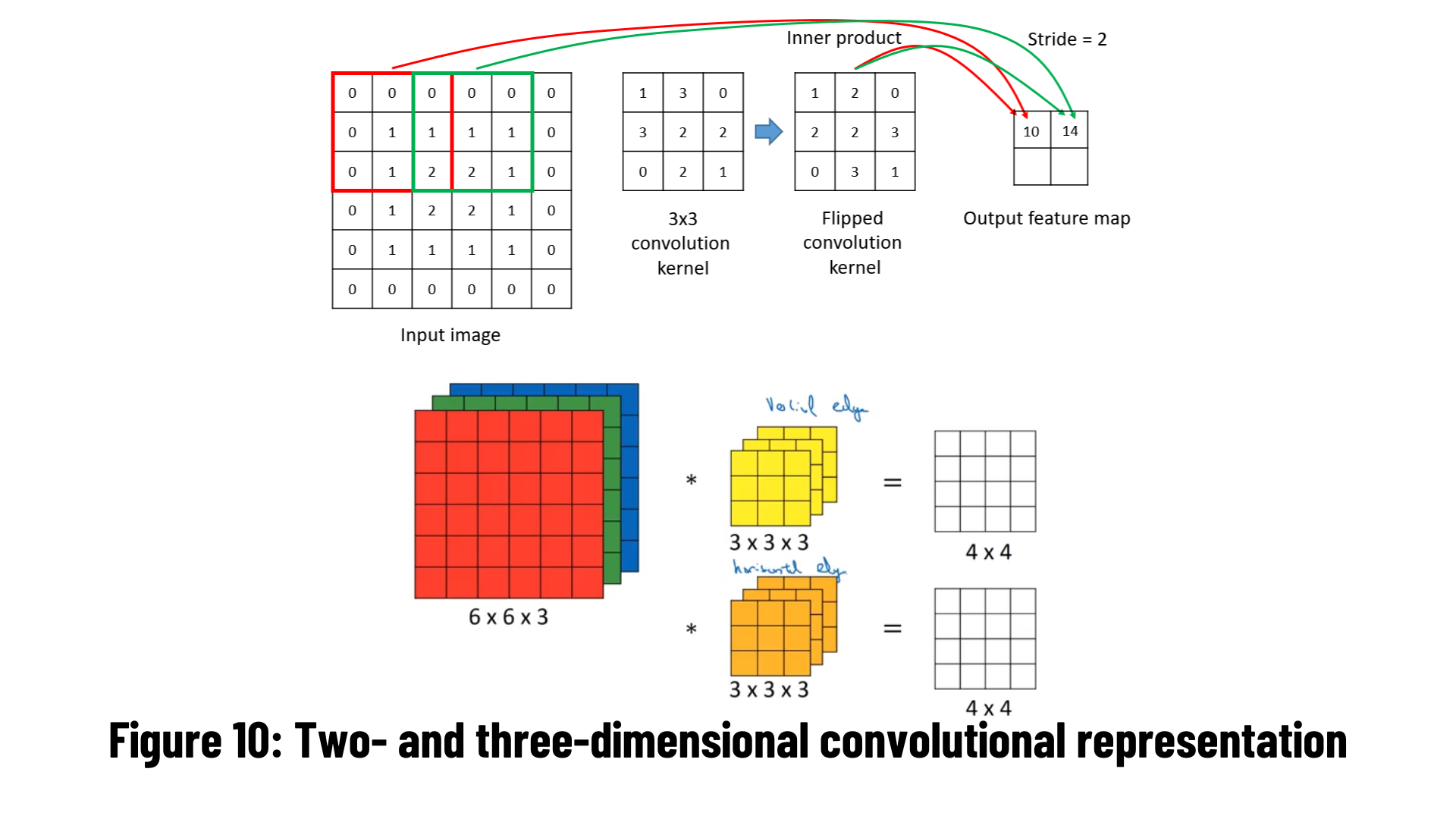
Color images consist of Red-Green-Blue (RGB) 3 channels. In this condition, the convolution operation is done for 3 channels. The channel number of the output signal is also calculated equally with the applied filter channel/number.
Let's imagine this computation process as a layer in a neural network. The input image and the filter are actually a matrix of weights that are constantly updated by backpropagation. A scalar b (bias) value is added last to the output matrix to which the activation function is applied. You can examine the convolution process flow from the image below.

Edge information is one of the most needed features from the image. It represents the high frequency regions of the input information. Two filters, vertical and horizontal, are used separately to obtain these attributes. In traditional methods - filters such as Sobel, Prewitt, Gabor - the filter is subject to a 'convolution' operation on the image. The resulting output shows the edge information of the image.

With different edge detection filters, angular edges, transitions from dark to light, and from light to dark are evaluated and calculated separately as an attribute. Generally, edges are computed in the first layers of a convolutional network model. While making all these calculations, there is a difference between the input size and the output size. For example; In case the input image (n): 6x6, edge detection filter (f): 3x3, the output image obtained as a result of the convolution operation becomes: (n-f+1)x(n-f+1)=4x4 dimensional. If it is not desired to reduce the size in this way - if the input and output sizes are desired to be equal - what should be done?
It is a computation at our disposal to manage the size difference between the input sign and the exit sign after the convolution operation. This is achieved by adding extra pixels to the input matrix.
This is exactly the job of adding pixels (padding) is called. In case the input matrix is nxn, filter (weight) matrix (fxf), if the output matrix is desired to be the same size as the input;
The formula (n+2p-f+1)x(n+2p-f+1) is applied.
Here, the value indicated by 'p' is the pixel size added to the input matrix, that is, the padding value. To determine this, the equation p=(f-1)/2 is used.
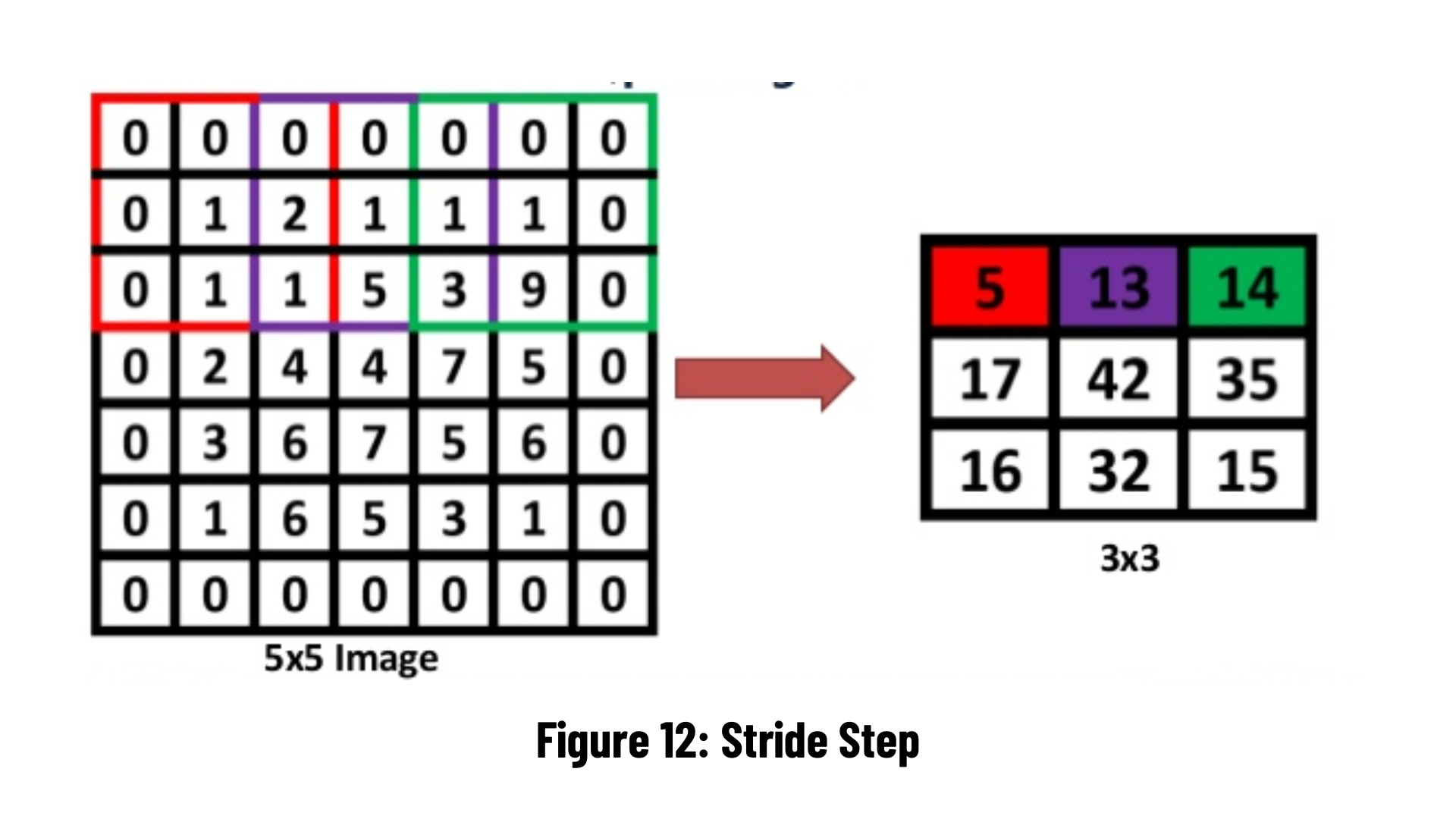
This value informs that for the convolution operation, the filter, which is the weight matrix, will shift on the image in one-pixel steps or larger steps. This is another parameter that directly affects the output size.
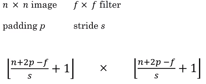 For example, when the padding value is p=1 and the number of steps is s=2, the size of the output matrix
(((n+2p-f)/s)+1)x(((n+2p-f)/s)+1);
If it is calculated for n=5 and f=3 values, the output size will be (3)x(3). Pixels added in the padding operation can consist of zeros, as in the example below. Another implementation is to copy the value of the next pixel.
In this layer, the maximum pooling method is generally used. There are no learned parameters in this layer of the network. It reduces the height and width information by keeping the number of channels of the input matrix constant. It is a step used to reduce computational complexity. However, according to Hinton's capsule theory, it compromises performance as it causes some important information in the data to be lost.
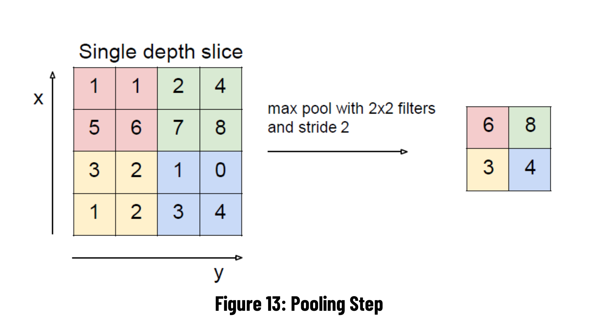
It gives very good results, especially in problems where location information is not very important. Outputs the largest of the pixels within the selected jointing size. In the example on the right, 2x2 max-commoning is applied by shifting it by 2 steps (pixels). The largest value in the field with the 4 related elements is transferred to the output. At the output, a 1 in 4 dimensional data is obtained.
We now know the operations performed in the context of a convolutional network. So how is the model created? The easiest answer to this question is to examine classical network models.
LeNet-5: It is the convolutional neural network model that was published in 1998 and gave the first successful result. It was developed by Yann LeCun and his team to read numbers on postal numbers, bank checks. Experiments are shown on the MNIST (Modified National Institute of Standards and Technology) dataset. In this model, unlike other models that will be developed later, average pooling is performed instead of max-pooling in size reduction steps. In addition, sigmoid and hyperbolic tangent are used as activation functions.
 The number of parameters entering the FC (Fully Connected) layer is 5x5x16=400 and there is a softmax with 10 classes because it classifies the numbers between 0 and 9 at the y output. In this network model, 60 thousand parameters are calculated. While the height and width information of the matrix decreases along the network, the depth (number of channels) value increases.
AlexNet: It is the first study that made convolutional neural network models and deep learning popular again in 2012. It was developed by Alex Krizhevsky, Ilya Sutskever and Geoffrey Hinton. It is basically very similar to the LeNet model in that it has successive layers of convolution and pooling. ReLU (Rectified Linear Unit) is used as an activation function, and max-pooling is used in pooling layers.
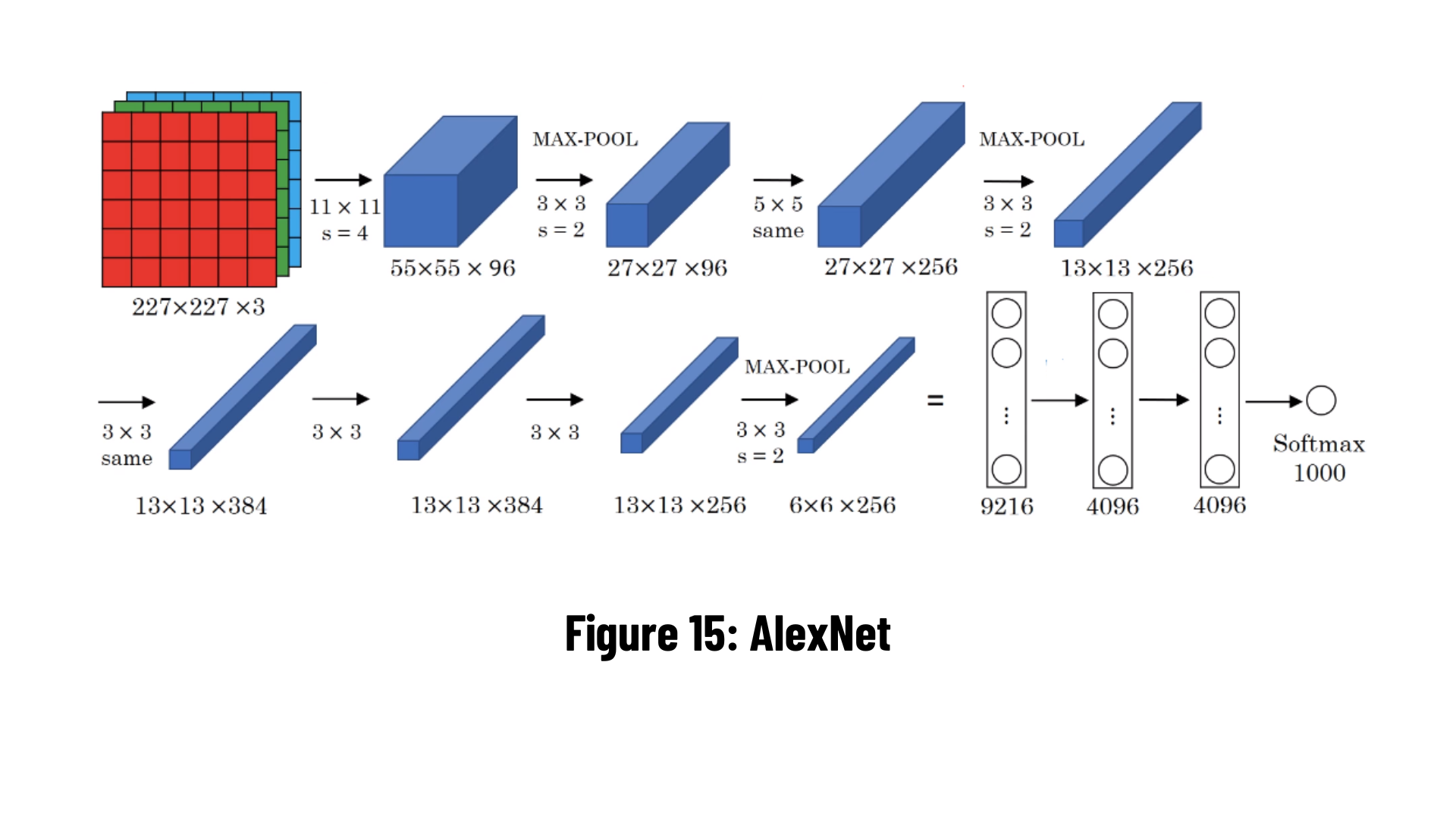 This larger and deeper network model is a two-part model on a parallel dual GPU (Graphics Processing Unit). Approximately 60 million parameters are calculated. It is a breaking point in the image classification problem, providing a spike in classification accuracy from 74.3% to 83.6% in the ImageNet ILSVRC competition.
VGG-16: It is a simple network model and the most important difference from the previous models is the use of convolution layers in 2 or 3 layers. It is converted into a feature vector with 7x7x512=4096 neurons in the full link (FC) layer. The 1000 class softmax performance is calculated at the output of the two FC layers. Approximately 138 million parameters are calculated. As in other models, while the height and width dimensions of the matrices decrease from the input to the output, the depth value (number of channels) increases.
 At each convolution layer output of the model, filters with different weights are calculated, and as the number of layers increases, the features formed in the filters represent the 'depths' of the image.
Other Common Network Architectures:
At each convolution layer output of the model, filters with different weights are calculated, and as the number of layers increases, the features formed in the filters represent the 'depths' of the image.
Other Common Network Architectures:
- GoogLeNet - 2014 ILSVRC winner, changing the network architecture and reducing the number of parameters (4 million instead of 60 milion in AlexNet)
- ResNet-50 - ResNet is one of the early adopters of batch normalisation (the batch norm paper authored by Ioffe and Szegedy was submitted to ICML in 2015) with 26M parameters.
- Inception-v1 - (2014) 22-layer architecture with 5M parameters
- Xception - It is an adaptation from Inception, where the Inception modules have been replaced with depthwise separable convolutions. It has also roughly the same number of parameters as Inception-v1.
Now let's look at object recognition algorithms using convolutional neural networks!!!
Object detection is a term related to computer vision and image processing that deals with detecting objects of a particular class (such as people, buildings or cars) in digital images and videos. More detailed explanation will be given in the following sections. Let's dive into R-CNN algorithm.
 R-CNN architecture has been developed because the CNN algorithm is not easily sufficient for images with multiple objects. The R-CNN algorithm uses the selective search algorithm that produces approximately 2000 possible regions where the object is likely to be found, and applies the CNN (ConvNet) algorithm to each region in turn. The size of the regions is determined and the correct region is placed in the neural network. A selective search algorithm is an algorithm that combines regions that are divided into smaller segments to generate a region recommendation.
Problems with R-CNN:
- Since each region in the image applies CNN separately, the training time is quite long and the prediction time is also long, so it takes a lot of time.
- A lot of disk space is required.
- The cost is high.
In R-CNN, we said that since the image is divided into 2000 regions, the training will take a lot of time and the cost will be high. Fast R-CNN was developed to solve this problem of R-CNN. The model consists of one stage compared to the 3 stages in R-CNN. It accepts only one image as input and displays the accuracy value of detected objects and bounding boxes. It also combines different parts of architectures (ConvNet, RoI Pooling Layer) into one complete architecture. This also eliminates the need to store a feature map and saves disk space.
Simply put, the ROI Pooling Layer applies maximum pooling to each cell (input) in the grid to generate fixed size feature maps.

Faster R-CNN, the most widely used and most advanced version of the R-CNN family, was first published in 2015. While both R-CNN and Fast R-CNN use CPU-based region bidding algorithms (For example: Selective search algorithm that takes about 2 seconds per image and runs on CPU computation), Faster R-CNN compares to Fast R-CNN to generate region suggestions. uses RPN, which is more convenient. This reduces the region suggest time from 2 seconds per image to 10 ms.
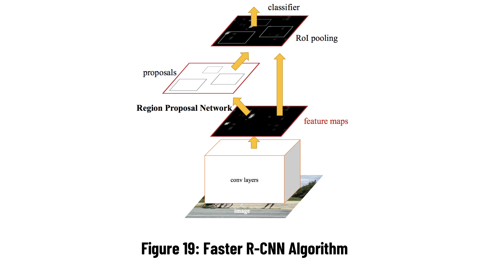
Region Proposal Network (RPN): The first stage, RPN, is a deep convolutional neural network for suggesting regions. The RPN takes any size of input as input and reveals the boundig box that can belong to a set of objects according to the truth value. It makes this suggestion by shifting a small mesh over the feature map generated by the convolutional layer.
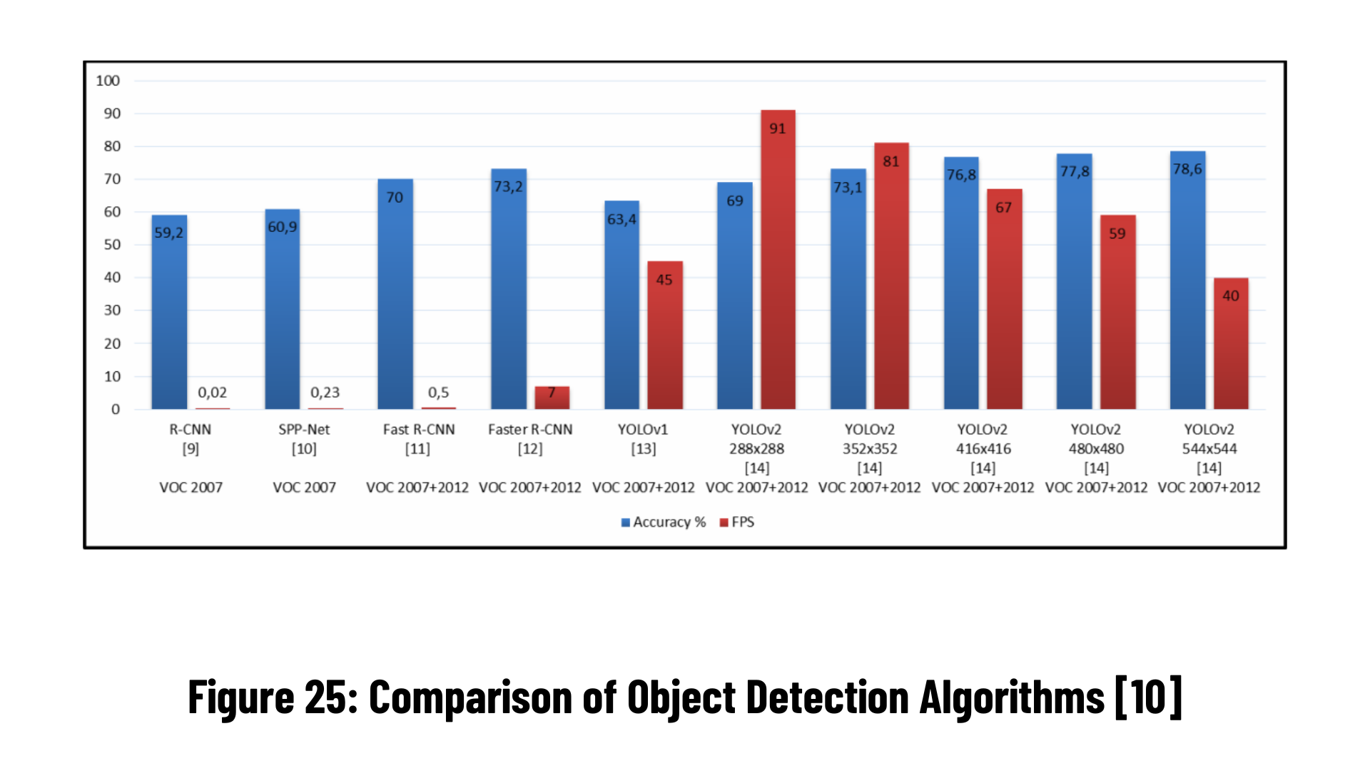
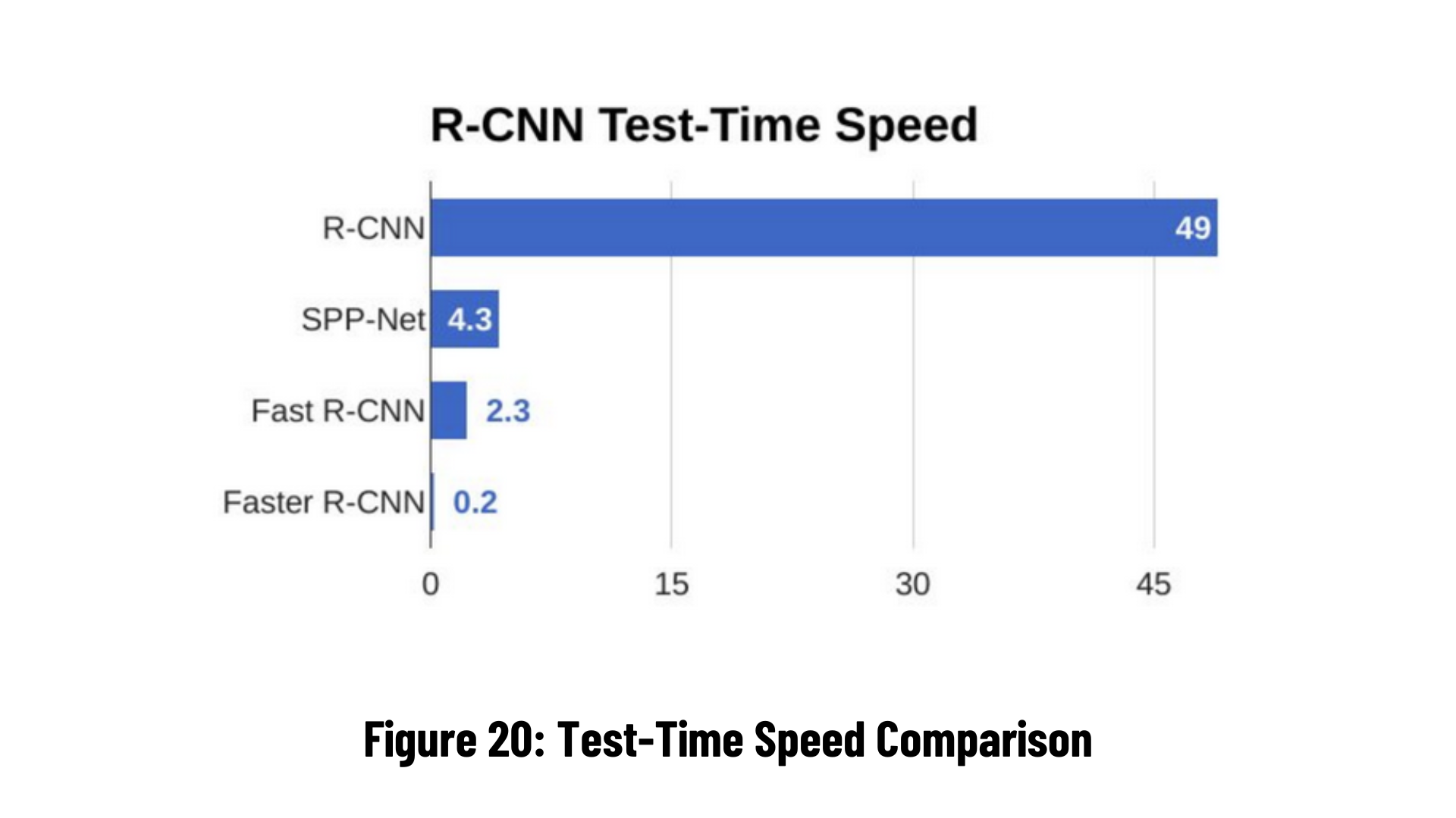 When the graph above is checked, you can notice that Faster R-CNN works in a much shorter time and is very fast. For this reason, Faster R-CNN is recommended for real-time object detection.
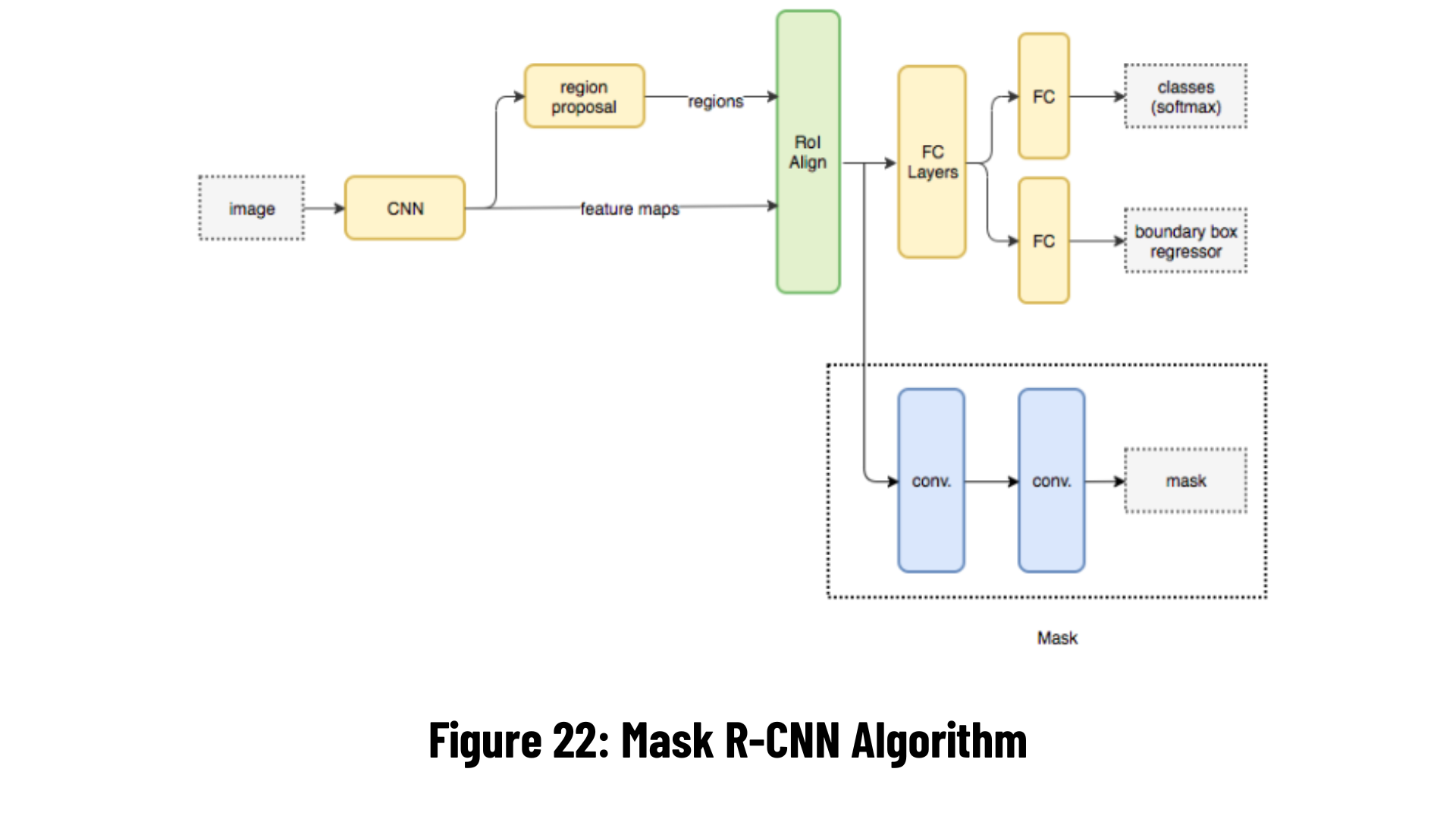
It is a deep neural network that aims to solve the instance segmentation problem in computer vision. Mask R-CNN can separate different objects in an image or video.
It is the task of defining object outlines at the pixel level. Compared to similar computer vision tasks, it is one of the most difficult vision tasks possible. If we consider the following tasks:

- Classification: There is a balloon in this image. Semantic
- Segmentation: These are all balloon pixels.
- Object Detection: There are 7 balloons at these locations in this image. (We started to account for overlapping objects.)
- Instance Segmentation: There are 7 balloons in these locations and these are the pixels of each.
Mask R-CNN (regional convolutional neural network) is a two-stage framework: the first stage scans the image and generates suggestions (areas that are most likely to contain an object). The second stage categorizes the suggestions and creates bounding boxes and masks. Both stages depend on the backbone structure.
 Here are the results of applications using Mask R-CNN in TensorFlow
Now let's talk about the most popular object detection algorithm of recent times. So why is the YOLO algorithm so popular?
- It is fast because it passes the image through the neural network in one go.
- High accuracy with minimum error.
- It has learning abilities that enable it to learn objects and apply them in object detection.
In fact, we aim to predict the bounding box that specifies the class of an object and the object location. Each bounding box can be defined by four attributes:
- Width (bw)
- height (bh)
- Class (e.g. person, car, traffic light, etc.)
- Bounding box center (bx,by)
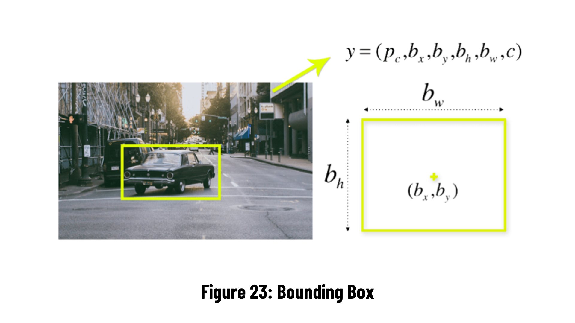
YOLO uses a single bounding box regression to estimate the height, width, center, and class of objects. The image above represents the accuracy probability (pc value) of an object appearing in the bounding box.
YOLO divides the input image into NxN grids. Each grid checks if there is an object in it and if the object thinks it exists, it checks whether the center point is in its area. Deciding that the object has a center point, the grid finds that object's class, height, and width and draws a bounding box around the object.
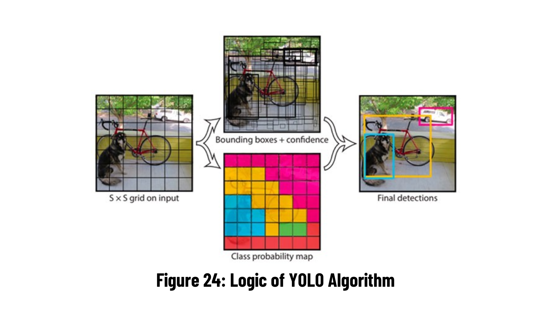
Sometimes the same object is repeatedly marked with a bounding box because it exists in more than one grid. As a solution, the Non-max Suppression algorithm draws the bounding boxes with the highest accuracy value on the screen for the objects detected on the image. In short, bounding boxes with accuracy values below the specified threshold are deleted.
The object detection technique Single Shot MultiBox Detector (SSD) is a version of the VGG16 architecture. It was made public at the end of November 2016 and broke previous performance and accuracy records for object detection tasks, earning over 74% mAP (mean Average Precision) at 59 frames per second on benchmark datasets including PascalVOC and COCO.
SSD’s architecture builds on the venerable VGG-16 architecture, but discards the fully connected layers.
The reason VGG-16 was used as the base network is because of its:
- strong performance in high quality image classification tasks
- popularity for problems where transfer learning helps in improving results
Instead of the original VGG fully connected layers, a set of auxiliary convolutional layers (from conv6 onwards) were added, thus enabling to extract features at multiple scales and progressively decrease the size of the input to each subsequent layer.
Region-based object detection algorithms such as R-CNN first determine the areas where objects are likely to be found and then apply CNN (Convolutional Neural Network, Convolutional Neural Networks) there separately. Although this method gives good results, since an image is subjected to two separate processes, the number of processing on the image increases and causes us to get a low FPS (Frames Per Second). The reason why the YOLO algorithm is so fast is that it can predict the class and coordinates of all objects in the picture by passing the image through the neural network at once, unlike systems such as R-CNN that require thousands of operations for a single image. So the basis of this estimation process is that they treat object detection as a single regression problem. This makes it extremely fast, 1000 times faster than R-CNN and 100 times faster than Fast R-CNN. If you need to do a project about real-time object detection, give the YOLO algorithm a chance.
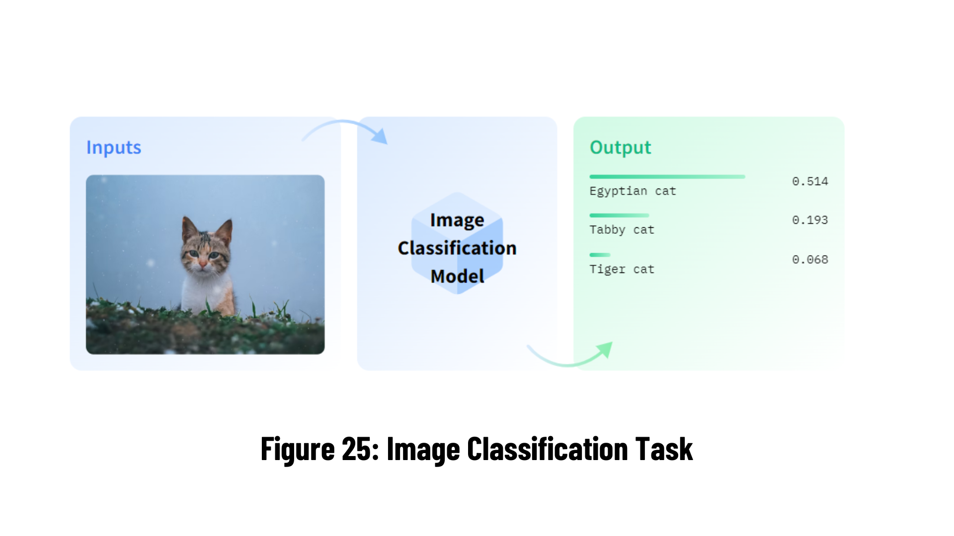
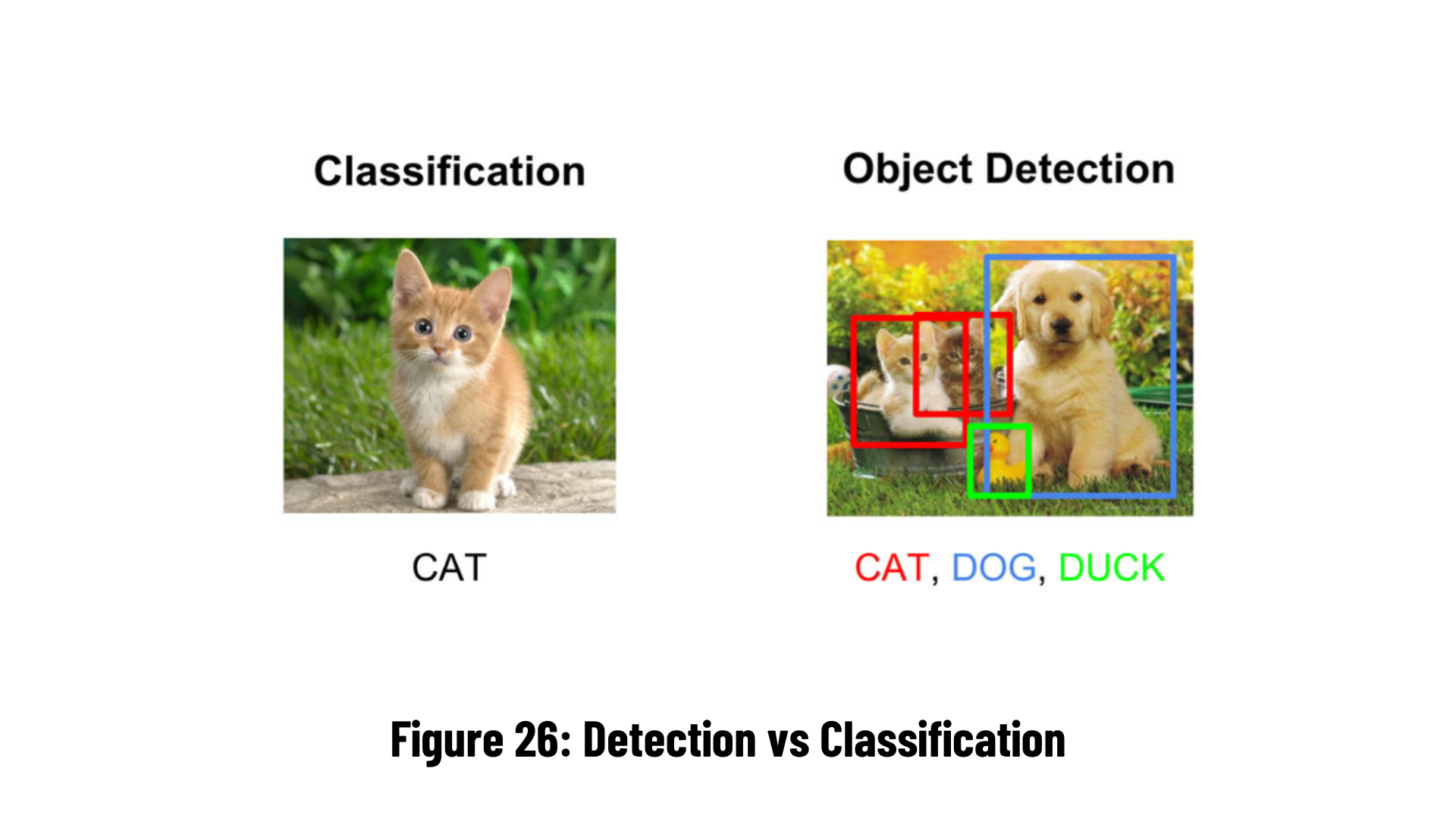
The process of classifying an entire image is known as image classification. It is assumed that each image will only have one class. The class to which an image belongs is predicted by image classification models when they receive an image as input.
- Satellite image classification
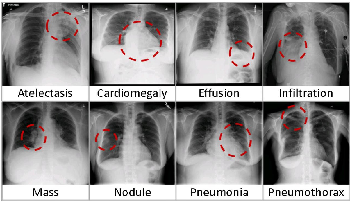
- Medical image classification
- Aircraft classification
- Chemical pattern classification
- Fault diagnosis
Object detection is a computer technology that deals with finding instances of semantic items of a specific class (such as individuals, buildings, or cars) in digital photos and videos. It is related to computer vision and image processing. Face detection and pedestrian detection are two well-studied object detection areas. Object detection can be used in a variety of computer vision applications, such as picture retrieval and video surveillance [11].
It's used for picture annotation, vehicle counting, activity recognition, face detection, face recognition, and video object co-segmentation, among other things. It's also used to track things, such as a ball during a football game, a cricket bat's movement, or a person in a film.
Every object class has its own unique characteristics that aid in classification - for example, all circles are round. These particular properties are used in object class detection. When looking for circles, for example, items at a specific distance from a point (i.e. the center) are sought. Similarly, objects that are perpendicular at corners and have equal side lengths are required while seeking for squares. Face identification uses a similar approach, with traits such as skin color and eye distance being detected along with the eyes, nose, and lips.
Object detection methods are classified as either neural network-based or non-neural approaches. Non-neural approaches require first defining features using one of the methods below, followed by classification using a technique such as support vector machine (SVM). On the other hand, neural approaches, which are often based on convolutional neural networks (CNN) , are capable of doing end-to-end object detection without specifying characteristics .
- Non-neural approaches:
- Neural network approaches:
- Region Proposals (R-CNN, Fast R-CNN, Faster R-CNN, cascade R-CNN).
- Single Shot MultiBox Detector (SSD)
- You Only Look Once (YOLO)
- Single-Shot Refinement Neural Network for Object Detection (RefineDet)
- Retina-Net
- Deformable convolutional networks
-
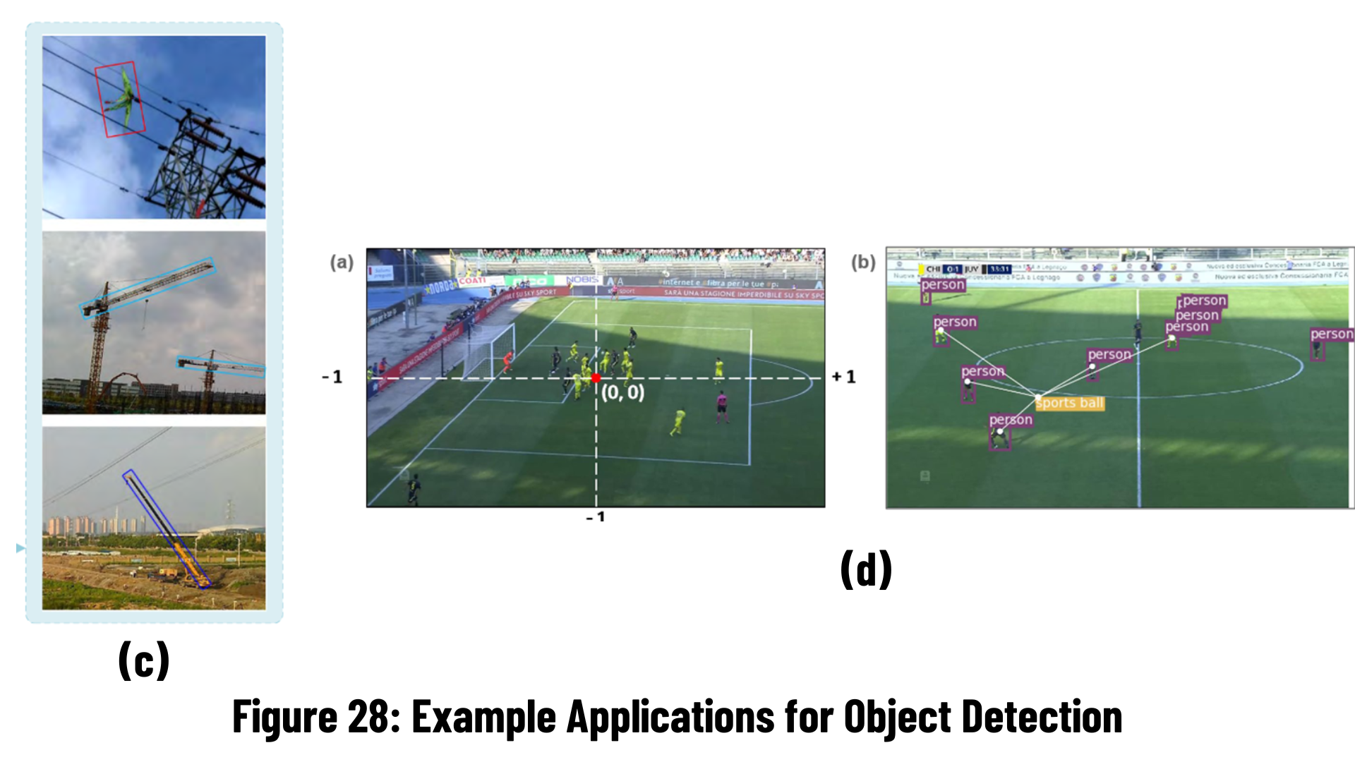
a. Automatic detection of earthquake-induced ground failure effects through Faster R-CNN deep learning-based object detection using satellite images [12].
-
b. Optical Braille Recognition Using Object Detection CNN [13].

-
c. A deep learning method to detect foreign objects for inspecting power transmission lines [14].
-
d. Automatic Pass Annotation from Soccer VideoStreams Based on Object Detection and LSTM [15].
Object recognition is a very popular computer vision technique used to detect as well as classify objects in images or videos. In short, this method includes object detection and classification.
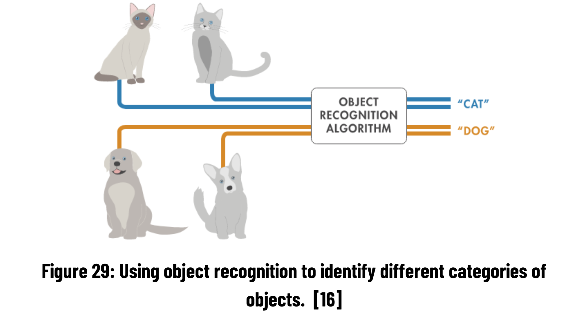
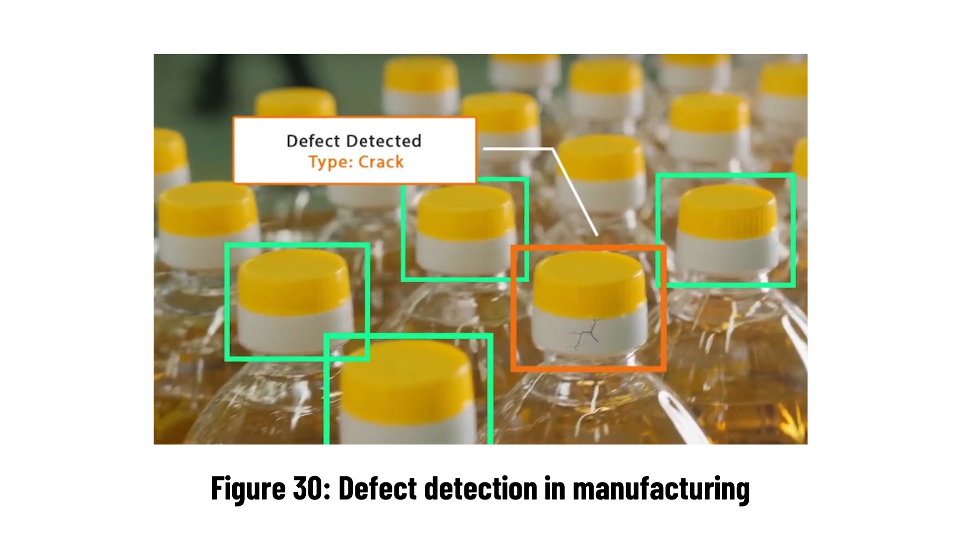
- a. Defect Detection (Manufacturing)
- b. Radiological imaging diagnostics
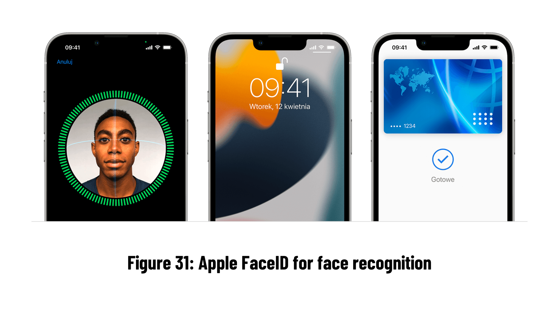
- c. Face recognition to identify and verify
It is aimed to follow the moving objects in the video and to obtain information such as location, speed or direction.
 Although people in videos are usually followed, animals or cars can also be followed. In order to carry out object tracking, object detection must be done first. Many different methods are used in object detection, such as subtracting two consecutive images from each other and detecting a moving object. Usually, after the objects in the image are detected, they are placed in a box and each box is assigned a number that has not been used before. Objects are tracked by these numbers.
Some challenges in object tracking:
- Unexpected disappearance of the tracked object.
- The tracked object then goes behind another object and is not visible.
- Detecting which is which when two objects intersect each other
- Detection of the same object even if the same object looks different due to the movement of the camera or the object itself.
- Objects can look very different from different perspectives and we need to consistently describe the same object from all perspectives.
- Objects in a video can change scale significantly, for example due to camera zoom. In this case, we need to recognize the same object.
- Light changes in video can have a huge impact on how objects appear and make it difficult to detect them consistently.
- a. Surveillance
- b. Traffic flow monitoring
- c. Autonomous Vehicles
- d. Human activity recognition
- e. Sports analytics
- f. Human counting
- Object Detection with Specific Color
- Motion Detection and Tracking with OpenCV
- Face and Eye Detection with OpenCV and Haar Feature based Cascade Classifiers
- MNIST Image Classification with Deep Neural Network
- MNIST Image Classification with Convolutional Neural Network
- Face Mask Detection for COVID19 with OpenCV, Tensorflow 2 and Keras
- Object Detection and Tracking in Custom Datasets with Yolov4
The goal here is fair self-explanatory:
- Step #1: Detect the presence of a colored object (blue in the code) using computer vision techniques.
- Step #2: Track the object as it moves around in the video frames, drawing its previous positions as it moves.
The end product should look similar to the GIF below:
Using HSV color range which is determined as Lower and Upper, I detected colorful object. Here I prefered blue objects.
# blue HSV
blueLower = (84,  98,  0)
blueUpper = (179, 255, 255)
When I got the color range, I set capture size and then I read the capture.
First I apply Gaussian Blurring for decreasing the noises and details in capture.
#blur
blurred = cv2.GaussianBlur(imgOriginal, (11,11), 0)
After Gaussian Blurring, I convert that into HSV color format.
# HSV
hsv = cv2.cvtColor(blurred, cv2.COLOR_BGR2HSV)
To detect Blue Object, I define a mask.
# mask for blue
mask = cv2.inRange(hsv, blueLower, blueUpper)
After mask, I have to clean around of masked object. Therefor I apply first Erosion and then Dilation
# deleting noises which are in area of mask
mask = cv2.erode(mask, None, iterations=2)
mask = cv2.dilate(mask, None, iterations=2)
After removing noises, the Contours have to be found
contours, _ = cv2.findContours(mask.copy(), cv2.RETR_EXTERNAL, cv2.CHAIN_APPROX_SIMPLE)
center = None
If the Contours have been found, I'll get the biggest contour due to be well.
# get max contour
c = max(contours, key=cv2.contourArea)
The Contours which are found have to be turned into rectangle deu to put rectangle their around. This cv2.minAreaRect() function returns a rectangle which is smallest to cover the area of object.
rect = cv2.minAreaRect(c)In the screen, we want to print the information of rectangle, therefore we need to reach its inform.
((x,y), (width, height), rotation) = rect
s = f"x {np.round(x)}, y: {np.round(y)}, width: {np.round(width)}, height: {np.round(height)}, rotation: {np.round(rotation)}"
Using this rectangle we found, we want to get a Box. In the next, we will use this Box for drawing Rectangle.
# box
box = cv2.boxPoints(rect)
box = np.int64(box)
Image Moment is a certain particular weighted average (moment) of the image pixels' intensities. To find Momentum, we use Max. Contour named as "c". After that, I find Center point.
# moment
M = cv2.moments(c)
center = (int(M["m10"] / M["m00"]), int(M["m01"] / M["m00"]))
Now, I will draw the center which is found.
# point in center
cv2.circle(imgOriginal, center, 5, (255, 0, 255), -1)
After Center Point, I draw Contour
# draw contour
cv2.drawContours(imgOriginal, [box], 0, (0, 255, 255), 2)
We want to print coordinators etc. in the screen
# print inform
cv2.putText(imgOriginal, s, (25, 50), cv2.FONT_HERSHEY_COMPLEX_SMALL, 1, (255, 255, 255), 2)
Finally, we wrote the code below to track the blue object with past data
# deque - draw the past data
        pts.appendleft(center)
        for i in range(1, len(pts)):
            if pts[i-1] is None or pts[i] is None: continue
            cv2.line(imgOriginal, pts[i-1], pts[i],(0,255,0),3) #
cv2.imshow("Original Detection",imgOriginal)The goal here is to find contours, draw contours and run a motion detection and tracking algorithm by using contour information.
The end product should look similar to the GIF below:
We may quickly locate items in a picture by using contour detection to locate their borders. It frequently serves as the starting point for a variety of fascinating applications, including picture-foreground extraction, basic image segmentation, detection, and recognition [17].
A contour is created by connecting every point along an object's boundaries. Typically, boundary pixels with the same color and intensity are referred to as a certain contour. Finding and drawing contours in images is quite simple with OpenCV. It does two straightforward tasks:
findContours()drawContours()
Also, it has two different algorithms for contour detection:
CHAIN_APPROX_SIMPLECHAIN_APPROX_NONE
Firstly, we captured the video that we have in our folder. These videos contain some walking people in Poznan, Paris and Rome. You can import any video by writing the name of the city by cap = cv2.VideoCapture('CITY_NAME.mp4').
print("Choose a City among Poznan, Paris or Rome")
print("-------------------------------------------")
cap = cv2.VideoCapture('paris.mp4') # Open the Video
Then, we want to read two frames from the capture.
out = cv2.VideoWriter("output.avi", fourcc, 5.0, (1280,720))
ret, frame1 = cap.read() # We define two frame one after another
ret, frame2 = cap.read()
We want to find the area that has changed since the last frame, not each pixel. In order to do so, we first need to find an area. This is what cv.findContours does; it retrieves contours or outer limits from each white spot from the part above. In the code below we find and draw all contours. Also, by using this contour information, we draw the rectangle to the object which are moving.
while cap.isOpened():
    diff = cv2.absdiff(frame1, frame2) # To find out absolute difference of first frame and second frame
    gray = cv2.cvtColor(diff, cv2.COLOR_BGR2GRAY) # convert it to gray scale - We do it for contour stages (It is easier to find contour with gray scale)
    blur = cv2.GaussianBlur(gray, (5,5), 0) # Blur the grayscale frame
    _, thresh = cv2.threshold(blur, 20, 255, cv2.THRESH_BINARY) # max threshold values is 255 - we need trashold value
    dilated = cv2.dilate(thresh, None, iterations=5)
    contours, _ = cv2.findContours(dilated, cv2.RETR_TREE, cv2.CHAIN_APPROX_SIMPLE) # Find contour
    for contour in contours:
        (x, y, w, h) = cv2.boundingRect(contour)

        if cv2.contourArea(contour) < 900:
            continue
        cv2.rectangle(frame1, (x, y), (x+w, y+h), (0, 255, 0), 2)
        cv2.putText(frame1, "Status: {}".format('Movement'), (10, 20), cv2.FONT_HERSHEY_SIMPLEX,
                    1, (0, 0, 255), 3) # If something is moving in the video then we will see Status: Movement
    #cv2.drawContours(frame1, contours, -1, (0, 255, 0), 2)
    image = cv2.resize(frame1, (1280,720))
    out.write(image)
    cv2.imshow("feed", frame1)
    frame1 = frame2
    ret, frame2 = cap.read()
    if cv2.waitKey(1) & 0xFF == ord('q'):
        break
cv2.destroyAllWindows()
cap.release()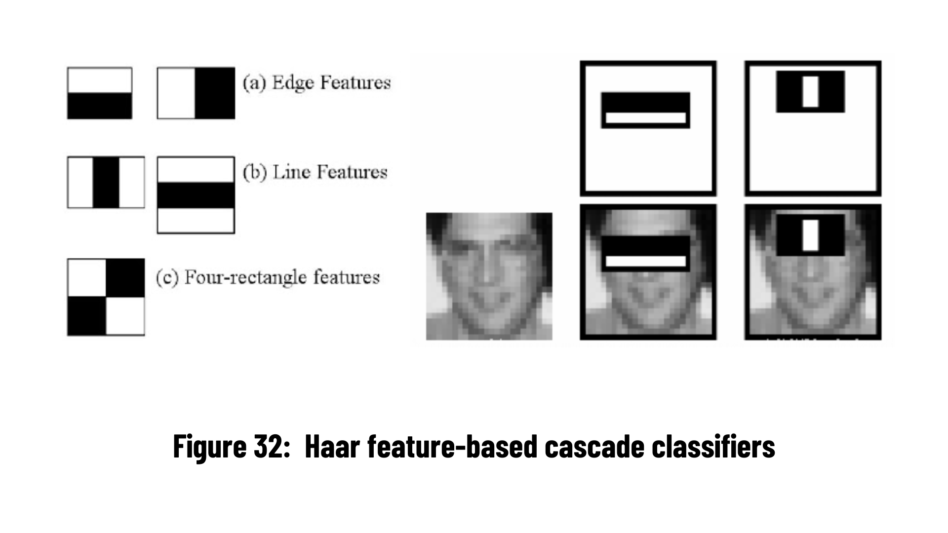
out.release()Paul Viola and Michael Jones in their study Rapid Object Detection using a Boosted Cascade of Simple Features [18] described an efficient object detection method that uses Haar feature-based cascade classifiers. We will detect face and eyes in this project by using Haar Cascade Classifiers.
The end product should look similar to the GIF below:

A cascade function is trained using a large number of both positive and negative images in this machine learning-based approach. The next step is to utilize it to find items in other pictures.
Face and eye detection will be used in this instance. To train the classifier, the algorithm first requires a large number of both positive (pictures of faces (and eyes)) and negative (images without faces (and eyes)). After that, we must draw features from it. The Haar features in the image below are utilized for this. They are just like convolutional kernel. Each feature is a single value that is obtained by deducting the sum of the pixels under the white and black rectangles.
At first we need to import pretrained models for face and eye detection so that we do not need to find a lot of photo with eyes, faces (positive) and without (negative). This will give us to save time.
In the following lines of the code we call these pretrained models by face_cascade, and eye_cascade.
import cv2

face_cascade = cv2.CascadeClassifier(cv2.data.haarcascades + 'haarcascade_frontalface_default.xml')
eye_cascade = cv2.CascadeClassifier(cv2.data.haarcascades + 'haarcascade_eye_tree_eyeglasses.xml')
Then we should choose video to capture (can be male or female). Next, we need to convert our image into grayscale because Haar cascades work only on gray images. So, we are going to detect faces and eyes in a grayscale images, but we will draw rectangles around the detected faces on the color images.
In the first step we will detect the face. To extract coordinates of a rectangle that we are going to draw around the detected face, we need to create object faces. In this object we are going to store our detected faces. With a function detectMultiScale() we will obtain tuple of four elements: x and y are coordinates of a top left corner, and w and h are width and height of the rectangle. This method requires several arguments. First one is the gray image, the input image on which we will detect faces. Second argument is the scale factor which tells us how much the image size is reduced at each image scale. Third and last argument is the minimal number of neighbors. This parameter specifying how many neighbors each candidate rectangle should have to retain it.
Later we detected the eyes. In order to do that, first we need to create two regions of interest Now we will detect the eyes. To detect the eyes, first we need to create two regions of interest which will be located inside the rectangle. We need first region for the gray image, where we going to detect the eyes, and second region will be used for the color image where we are going to draw rectangles.
print("Enter Female Face or Male Face")
cap = cv2.VideoCapture('female.mp4')

while cap.isOpened():
    _, img = cap.read()
    gray = cv2.cvtColor(img, cv2.COLOR_BGR2GRAY)
    faces = face_cascade.detectMultiScale(gray, 1.1, 4)

    for (x, y , w ,h) in faces:
        cv2.rectangle(img, (x,y), (x+w, y+h), (255, 0 , 0), 3)
        roi_gray = gray[y:y+h, x:x+w]
        roi_color = img[y:y+h, x:x+w]
        eyes = eye_cascade.detectMultiScale(roi_gray)
        for (ex, ey ,ew, eh) in eyes:
            cv2.rectangle(roi_color, (ex,ey), (ex+ew, ey+eh), (0, 255, 0), 5)

    # Display the output
    cv2.imshow('img', img)
    if cv2.waitKey(1) & 0xFF == ord('q'):
        break

cap.release()Click Here for Detailed Information
Click Here for Detailed Information
In this project, it is aimed to create a Convolutional Neural Network to classify the digits from 0 to 9. Approximately 10000 images from 10 different classes are trained in the training code. A test script was then created for use with a webcam.
The end product should look similar to the GIF below:
Let's dive into the codes:
train_cnn.py:
The code below is for reading the images as well as the labels.
path = "digits_data"
myList = os.listdir(path)
noOfClasses = len(myList)
print("Number of Label/Class: ",noOfClasses)
images = []
classNo = []
#### IMPORTING DATA/IMAGES FROM FOLDERS
for i in range(noOfClasses):
    myImageList = os.listdir(path + "\\"+str(i))
    for j in myImageList:
        img = cv2.imread(path + "\\" + str(i) + "\\" + j)
        img = cv2.resize(img, (32,32))
        images.append(img)
        classNo.append(i)
Then we split our dataset into train, test and validation.
x_train, x_test, y_train, y_test = train_test_split(images, classNo, test_size = 0.3, random_state = 42)
x_train, x_validation, y_train, y_validation = train_test_split(x_train, y_train, test_size = 0.2, random_state = 42)
We can see the distribution of the test, train and validation via code below.
fig, axes = plt.subplots(3,1,figsize=(7,7))
fig.subplots_adjust(hspace = 0.5)
sns.countplot(y_train, ax = axes[0])
axes[0].set_title("y_train")

sns.countplot(y_test, ax = axes[1])
axes[1].set_title("y_test")

sns.countplot(y_validation, ax = axes[2])
axes[2].set_title("y_validation")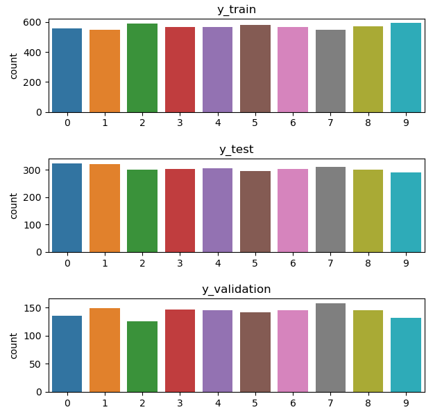
Next, preprocessing function needs to be created to properly train our images with CNN.
def preProcess(img):
    img = cv2.cvtColor(img, cv2.COLOR_BGR2GRAY)
    img = cv2.equalizeHist(img)
    img = img /255
    return img
Later, we reshape your images and apply data augmentation for creating more variety of data, which helps us to learn better.
x_train = x_train.reshape(-1,32,32,1)
print(x_train.shape)
x_test = x_test.reshape(-1,32,32,1)
x_validation = x_validation.reshape(-1,32,32,1)

dataGen = ImageDataGenerator(width_shift_range = 0.08,
                             height_shift_range = 0.08,
                             zoom_range = 0.08,
                             rotation_range = 8)

dataGen.fit(x_train)
Before training the model, output variable should be implemented one hot encoding and then we can create model and apply CNN algorithm. Finally, we save our model for further real time classification.
y_train = to_categorical(y_train, noOfClasses)
y_test = to_categorical(y_test, noOfClasses)
y_validation = to_categorical(y_validation, noOfClasses)
model = Sequential()
model.add(Conv2D(input_shape = (32,32,1), filters = 8, kernel_size = (5,5), activation = "relu", padding = "same"))
model.add(MaxPooling2D(pool_size = (2,2)))
model.add(Conv2D( filters = 16, kernel_size = (3,3), activation = "relu", padding = "same"))
model.add(MaxPooling2D(pool_size = (2,2)))
model.add(Dropout(0.2))
model.add(Flatten())
model.add(Dense(units=256, activation = "relu" ))
model.add(Dropout(0.2))
model.add(Dense(units=noOfClasses, activation = "softmax" ))
model.compile(loss = "categorical_crossentropy", optimizer=("Adam"), metrics = ["accuracy"])
batch_size = 64
hist = model.fit_generator(dataGen.flow(x_train, y_train, batch_size = batch_size),
validation_data = (x_validation, y_validation),
epochs = 30,steps_per_epoch = x_train.shape[0]//batch_size, shuffle = 1)
model_json = model.to_json()
with open("model.json", "w") as json_file:
json_file.write(model_json)
# serialize weights to HDF5
model.save_weights("model_trained.h5")
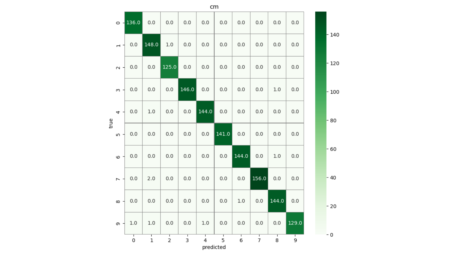
print("Saved model to disk")Finally, we plot our results and see confusiton matrix.
plt.figure()
plt.plot(hist.history["loss"], label = "Train Loss")
plt.plot(hist.history["val_loss"], label = "Validation Loss")
plt.legend()
plt.show()

plt.figure()
plt.plot(hist.history["accuracy"], label = "Train accuracy")
plt.plot(hist.history["val_accuracy"], label = "Validation accuracy")
plt.legend()
plt.show()

score = model.evaluate(x_test, y_test, verbose = 1)
print("Test loss: ", score[0])
print("Test accuracy: ", score[1])

y_pred = model.predict(x_validation)
y_pred_class = np.argmax(y_pred, axis = 1)
Y_true = np.argmax(y_validation, axis = 1)
cm = confusion_matrix(Y_true, y_pred_class)
f, ax = plt.subplots(figsize=(8,8))
sns.heatmap(cm, annot = True, linewidths = 0.01, cmap = "Greens", linecolor = "gray", fmt = ".1f", ax=ax)
plt.xlabel("predicted")
plt.ylabel("true")
plt.title("cm")
plt.show()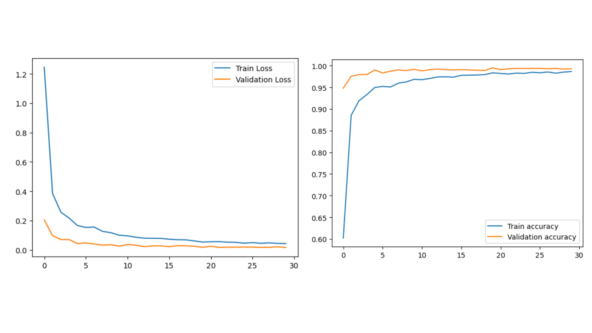
video_capture.py:
The code below is for capturing the video, loading the saved model and classifiying the digit in real time.
import cv2
import numpy as np
from tensorflow.keras.models import model_from_json

#### PREPORCESSING FUNCTION
def preProcess(img):
    img = cv2.cvtColor(img, cv2.COLOR_BGR2GRAY)
    img = cv2.equalizeHist(img)
    img = img /255.0
    return img

#### CREATE CAMERA OBJECT
cap = cv2.VideoCapture(0)
cap.set(3,480)
cap.set(4,480)

### load json and create model
json_file = open('model.json', 'r')
loaded_model_json = json_file.read()
json_file.close()
model = model_from_json(loaded_model_json)
### load weights into new model
model.load_weights("model_trained.h5")
print("Loaded model from disk")

while True:
    success, frame = cap.read()
    img = np.asarray(frame)
    img = cv2.resize(img, (32,32))
    img = preProcess(img)
    img = img.reshape(1,32,32,1)
    #### PREDICT
    classIndex = int(model.predict_classes(img))
    predictions = model.predict(img)
    probVal = np.amax(predictions)
    print(classIndex, probVal)
    if probVal > 0.7:
        cv2.putText(frame, str(classIndex)+ "   "+ str(probVal), (50,50),cv2.FONT_HERSHEY_DUPLEX, 1,(0,255,0),1)
    cv2.imshow("Digit Classification",frame)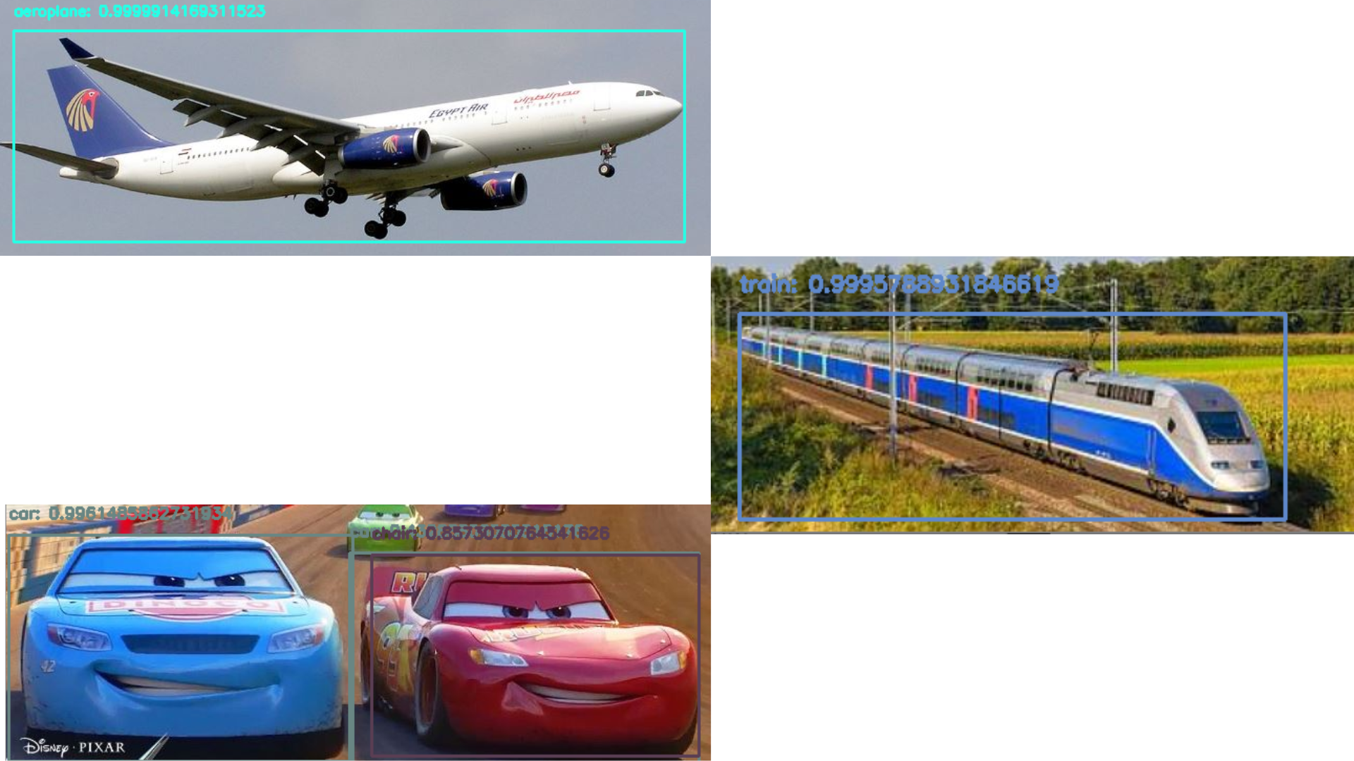
if cv2.waitKey(1) & 0xFF == ord("q"): break In this project, it is aimed to use MobileNets + Single Shot Detectors along with OpenCV to perform deep learning based real time object recognition.
The end product should look similar to the GIF below:
There are two pyton file in this project. One of them (real_time.python) is for real time recognition and the other (recognition with mobilenet and ssd.py) is for image based recognion.
Some of the outputs of image based recognition:
Since we learned the basics of computer vision and image processing thanks to this project, we are planning to test them on a mobile robot with a camera and make a project that can detect objects in real time and take different actions as a result of the detections.
- [1] - https://peakup.org/blog/yeni-baslayanlar-icin-goruntu-islemeye-giris/
- [2] - https://yapayzeka.itu.edu.tr/arastirma/bilgisayarla-goru
- [3] - VBM686 – Computer Vision Pinar Duygulu Hacettepe University Lecture Notes
- [4] - O’Mahony, N.; Campbell, S.; Carvalho, A.; Harapanahalli, S.; Velasco-Hernandez, G.; Krpalkova, L.; Riordan, D.; Walsh, J. Deep Learning vs. Traditional Computer Vision. arXiv 2019, arXiv:1910.13796.
- [5] - https://towardsdatascience.com/the-differences-between-artificial-and-biological-neural-networks-a8b46db828b7
- [6] - https://pytorch.org/
- [7] - https://keras.io/
- [8] - https://docs.fast.ai/
- [9] - https://www.coursera.org/specializations/deep-learning
- [10] - Ceren Gulra Melek, Elena Battini Sonmez, and Songul Albayrak, “Object Detection in Shelf Images with YOLO” 978-1-5386-9301-8/19/$31.00 ©2019 IEEE, 2019, doi: 10.1109/EUROCON.2019.8861817
- [11] - https://en.wikipedia.org/wiki/Object_detection
- [12] - Hacıefendioğlu, K., Başağa, H.B. & Demir, G. Automatic detection of earthquake-induced ground failure effects through Faster R-CNN deep learning-based object detection using satellite images. Nat Hazards 105, 383–403 (2021). https://doi.org/10.1007/s11069-020-04315-y
- [13] - Ovodov, I. G. (2020). Optical Braille Recognition Using Object Detection CNN. ArXiv:2012.12412.
- [14] - J. Zhu et al., "A Deep Learning Method to Detect Foreign Objects for Inspecting Power Transmission Lines," in IEEE Access, vol. 8, pp. 94065-94075, 2020, doi: 10.1109/ACCESS.2020.2995608.
- [15] - Danilo Sorano, Fabio Carrara, Paolo Cintia, Fabrizio Falchi, and Luca Pappalardo. Automatic pass annotation from soccer videostreams based on object detection and lstm. arXiv preprint arXiv:2007.06475, 2020.
- [16] - https://www.mathworks.com/solutions/image-video-processing/object-recognition.html
- [17] - https://learnopencv.com/contour-detection-using-opencv-python-c/
- [18] - P. Viola and M. Jones, "Rapid object detection using a boosted cascade of simple features," Proceedings of the 2001 IEEE Computer Society Conference on Computer Vision and Pattern Recognition. CVPR 2001, 2001, pp. I-I, doi: 10.1109/CVPR.2001.990517.