Detailed Consideration of Artificial Neural Networks on Letter and Image Recognition Project Using Matlab Program
Author: Turhan Can Kargın
Software: MATLAB
This repository is my assignments on Basics of Smart Systems Laboratory Class which I took during my master degree at Poznan University of Technology. I share this with you to help you to basic understanding of artiicial neural network theory and application on MATLAB.

Artificial neural networks are becoming widely used in many areas such as complex robotics problems, computer vision, and classification problems. Working on artificial neural networks commonly referred to as “neural networks”, has been motivated right from its inception by the recognition that the human brain computes in an entirely different way from the conventional digital computer. The brain is highly complex, nonlinear and parallel computer. It has capability to organize its structural constituents, known as neurons, so as to perform certain computations (such as perception and motor control) very fast. Therefore, the interest of artificial neural network is to perform useful computations through a process of learning like our brain. This report presents how artificial neural networks can be used in letter recognition and image recognition. The report is broadly categorized into two; the first part is a short overview on artificial neural networks, particularly its generalization property, as applied to systems identification. Second part contains some experimental design which shows how we can obtain neural network into applications.
Neural networks are closely modeled on biological processes for information processing, including specifically the nervous system and its basic unit, the neuron. Signals are propagated in the form of potential differences between the inside and outside of cells. The main components of a neuronal cell are shown in Figure 1. Dendrites bring signals from other neurons into the cell body or soma, possibly multiplying each incoming signal by a transfer weighting coefficient. In the soma, cell capacitance integrates the signals which collect in the axon hillock. Once the composite signal exceeds a cell threshold, a signal, the action potential, is transmitted through the axon. Cell nonlinearities make the composite action potential a nonlinear function of the combination of arriving signals. The axon connects through synapses with the dendrites of subsequent neurons. The synapses operate through the discharge of neurotransmitter chemicals across intercellular gaps, and can be either excitatory (tending to fire the next neuron) or inhibitory (tending to prevent firing of the next neuron) [1].
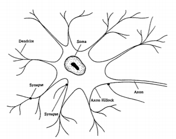
Figure 1 - Neuron Anatomy
Neural networks are set of algorithms inspired by the functioning of human brian. Generally when you open your eyes, what you see is called data and is processed by the Neurons (data processing cells) in your brain, and recognizes what is around you. That’s how similar the Neural Networks works. They takes a large set of data, process the data (draws out the patterns from data), and outputs what it is. What they do? Neural networks sometimes called as Artificial Neural networks (ANN’s), because they are not natural like neurons in your brain. They artificially mimic the nature and functioning of neural network. ANN’s are composed of a large number of highly interconnected processing elements (neurons) working in unison to solve specific problems. ANNs, like people, like child, they even learn by example. An ANN is configured for a specific application, such as pattern recognition or data classification, image recognition, voice recognition through a learning process. Neural networks, with their remarkable ability to derive meaning from complicated or imprecise data, can be used to extract patterns and detect trends that are too complex to be noticed by either humans or other computer techniques. A trained neural network can be thought of as an “expert” in the category of information it has been given to analyse. This expert can then be used to provide projections given new situations of interest and answer “what if” questions. Other advantages include:
- Adaptive learning: An ability to learn how to do tasks based on the data given for training or initial experience.
- Self-Organization: An ANN can create its own organization or representation of the information it receives during learning time.
The most common type of artificial neural network consists of three groups, or layers, of units: a layer of “input” units is connected to a layer of “hidden” units, which is connected to a layer of “output” units.
- Input units - The activity of the input units represents the raw information that is fed into the network. This also called input layer.
- Hidden units - The activity of each hidden unit is determined by the activities of the input units and the weights on the connections between the input and the hidden units. This also called hidden layer.
- Output units - The behavior of the output units depends on the activity of the hidden units and the weights between the hidden and output units. this also called output layer.
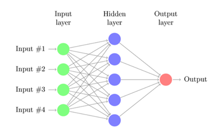
Figure 2 - Neural Network with Input, Hidden and Output layer [2]
So the circles are called neurons. One list of neurons is a layer: the first layer is the input layer, while the last one (in our case, represented by only one neuron) is the output layer; those in the middle, on the other hand, are the hidden layers. Finally, all the interconnections among neurons are our synapses. The main elements of NN are, in conclusion, neurons and synapses, both in charge of computing mathematical operations. Yes, because NNs are nothing but a series of mathematical computations: each synapsis holds a weight, while each neuron computes a weighted sum using input data and synapses’ weights [3].
Perceptrons — invented by Frank Rosenblatt in 1958, are the simplest neural network that consists of n number of inputs, only one neuron, and one output, where n is the number of features of our dataset. The process of passing the data through the neural network is known as forward propagation and the forward propagation carried out in a perceptron is explained in the following three steps.
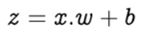
Step 1: For each input, multiply the input value xᵢ with weights wᵢ and sum all the multiplied values. Weights — represent the strength of the connection between neurons and decide how much influence the given input will have on the neuron’s output. If the weight w₁ has a higher value than the weight w₂, then the input x₁ will have a higher influence on the output than w₂.

The row vectors of the inputs and weights are x = [x1, x2, … , xn] and w =[w1, w2, … , wn] respectively and their dot product is given by

Hence, the summation is equal to the dot product of the vectors x and w

Step 2: Add bias b to the summation of multiplied values and let’s call this z. Bias — also known as the offset is necessary in most of the cases, to move the entire activation function to the left or right to generate the required output values.
Step 3: Pass the value of z to a non-linear activation function. Activation functions — are used to introduce non-linearity into the output of the neurons, without which the neural network will just be a linear function. Moreover, they have a significant impact on the learning speed of the neural network. Perceptrons have binary step function as their activation function. However, we shall use sigmoid — also known as logistic function as our activation function.
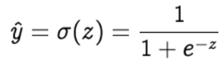
where σ denotes the sigmoid activation function and the output we get after the forward prorogation is known as the predicted value ŷ.
The learning algorithm consists of two parts — backpropagation and optimization.
Backpropagation, short for backward propagation of errors, refers to the algorithm for computing the gradient of the loss function with respect to the weights. However, the term is often used to refer to the entire learning algorithm. The backpropagation carried out in a perceptron is explained in the following two steps.
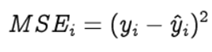
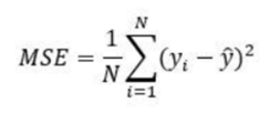
Step 1: To know an estimation of how far are we from our desired solution a loss function is used. Generally, mean squared error is chosen as the loss function for regression problems and cross entropy for classification problems. Let’s take a regression problem and its loss function be mean squared error, which squares the difference between actual (yᵢ) and predicted value (ŷᵢ ).
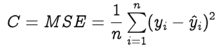
Loss function is calculated for the entire training dataset and their average is called the Cost function C.
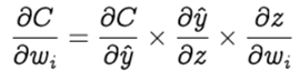
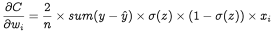
Step 2: In order to find the best weights and bias for our Perceptron, we need to know how the cost function changes in relation to weights and bias. This is done with the help of the gradients (rate of change) — how one quantity changes in relation to another quantity. In our case, we need to find the gradient of the cost function with respect to the weights and bias. Let’s calculate the gradient of cost function C with respect to the weight wᵢ using partial derivation. Since the cost function is not directly related to the weight wᵢ, let’s use the chain rule.
Now we need to find the following three gradients
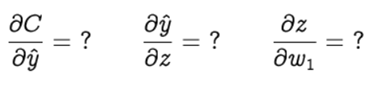
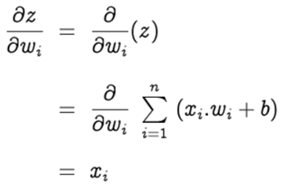
Let’s start with the gradient of the cost function (C) with respect to the predicted value ( ŷ )
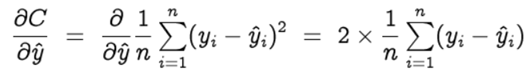
Let y = [y1 , y2 , … yn] and ŷ =[ ŷ1 , ŷ2 , … ŷn] be the row vectors of actual and predicted values. Hence the above equation is simplified as
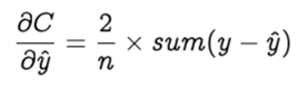
Now let’s find the gradient of the predicted value with respect to the z. This will be a bit lengthy.
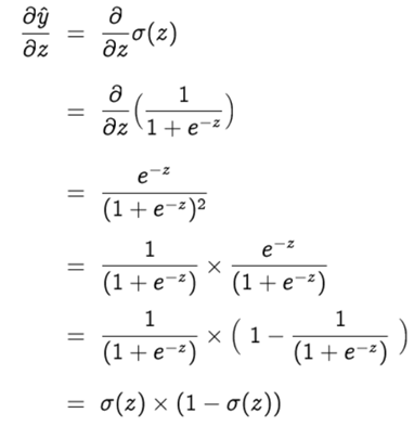
The gradient of z with respect to the weight wᵢ is
Therefore we get,
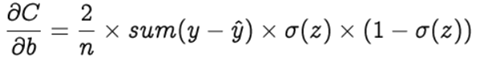
What about Bias? — Bias is theoretically considered to have an input of constant value 1. Hence,
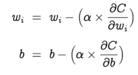
Optimization is the selection of the best element from some set of available alternatives, which in our case, is the selection of best weights and bias of the perceptron. Let’s choose gradient descent as our optimization algorithm, which changes the weights and bias, proportional to the negative of the gradient of the cost function with respect to the corresponding weight or bias. Learning rate (α) is a hyperparameter which is used to control how much the weights and bias are changed. The weights and bias are updated as follows and the backpropagation and gradient descent is repeated until convergence [4].
I have explained the working of a single neuron in the introduction part of this report. However, these basic concepts are applicable to all kinds of neural networks with some modifications. Now, let’s tell our materials for the projects and start to explain the experimental design. I will talk about first how to create a neural network in MATLAB and then I will explain three different projects which are letter recognition and image recognition with Neural Network in the experimental design part of the report.
In this part of the report I want to explain what we did in these projects, what is the design process, our MATLAB code and our Simulink results. Firstly, I will start with brief introduction to neural network toolbox for MATLAB.
%% Introduction
% Brief Introduction To Neural Network Toolbox for Matlab
% Simple example: how to prepare teaching data, create the neural network,
% train it and simulate.
clc
clear all
%%
% Create teaching input vector:
P = [0 1 2 3 4 5 6 7 8 9 10];
% teaching output vector (so called target vector):
T = [0 1 2 3 4 3 2 1 2 3 4];
% Values in P and T vectors are pairs: T(n) is expected output value for input P(n).
%%
% Create 'clean' network
net = newff([0 10],[5 1],{'tansig' ,'purelin'});
% See the description of the newff function parameters by typing:
help newff
% Set the number of teaching epochs:
net.trainParam.epochs = 50;
% and train the network:
[net, tr, Y, E] = train(net,P,T);
% See description of the train function parameters by typing:
help train
% Now you can simulate the network (check the response of the neural network):
A = sim(net, P);
% Neural network can be saved to file just like any other variable or object in Matlab.
%%
% Review transition functions available in the toolbox:
n = -5:0.1:5;
plot(n,hardlim(n),'r+:');
% Plot the following functions: purelin, logsig, tansig, satlin.
Figure 3 - Introduction Code
In the Figure below, we introduced how to create neural network on Matlab. Now, I will explain every line one by one. We created 1x11 vector for teaching input in line 7. After that, we created again 1x11 vector for teaching output in line 9. Later, in line 13 free neural network was created. It has [0 10] input vector and [5 1] output vector. ‘tansig’ means that first activation function is hyperbolic tangent sigmoid transfer function (Figure 4) and ‘purelin’ means that second activation function is linear transfer function (Figure 4).
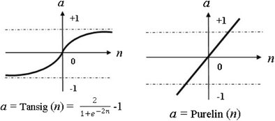
Figure 4 - tansig and purelin
net.trainParam.epochs = 50; is for number of teaching the network which means epoch number. In this case we decided 50 times.
at [net, tr, Y, E] = train(net,P,T); section, we finally trained the neural network with 50 epoch. Finally, we can check our accuracy and simulate our network as A = sim(net, P); You can see our simulated network in Figure 5.
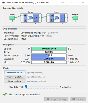
Figure 5 - Trained Network
Now let’s check the performance (Figure 6). As you see in Figure 6, we reached the best performance at 28th epoch. So, we can adjust our epoch number to 28 so that it will be more efficient. Last rows on the code shows that how to visualize the activation functions. In our code it show the step function (hardlim). But we can also visualize other functions like tansig and purelim (Figure 7)
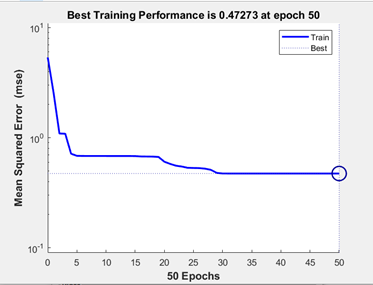
Figure 6 – Performance
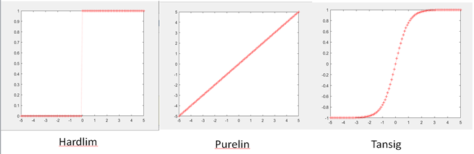
Figure >7 - Activation Function Visualization
Now that we have explained how we create an artificial neural network with Matlab, we can begin to describe our first project.

In this project, our aim is to give every English Letter to the neural network in the form of binary, train them and finally correctly predict the letters after training. Let’s first check our MATLAB code one by one. Firstly input vectors were defined as shown in Figure 8. We define letters as binary vectors. Let me explain how we made this binary form. The letters were defined as 7x5 pixel (matrix). When we draw a B letter on a 7x5 image, we obtain something like a left side picture. Black pixels mean “1” and white pixels mean “0”. Therefore, if we want this image to transform into binary form, we obtain “PB = [1 1 1 1 0 1 0 0 0 1 1 0 0 0 1 1 1 1 1 0 1 0 0 0 1 1 0 0 0 1 1 1 1 1 0]”. The same processes were applied for all English Letters as shown in Figure 8.
%% Input Vectors
PA = [0 1 1 1 0  1 0 0 0 1  1 0 0 0 1  1 0 0 0 1  1 1 1 1 1  1 0 0 0 1  1 0 0 0 1];
PB = [1 1 1 1 0  1 0 0 0 1  1 0 0 0 1  1 1 1 1 0  1 0 0 0 1  1 0 0 0 1  1 1 1 1 0];
PC = [0 1 1 1 0  1 0 0 0 1  1 0 0 0 0  1 0 0 0 0  1 0 0 0 0  1 0 0 0 1  0 1 1 1 0];
PD = [1 1 1 0 0  1 0 0 1 0  1 0 0 0 1  1 0 0 0 1  1 0 0 0 1  1 0 0 1 0  1 1 1 0 0];
PE = [1 1 1 1 1  1 0 0 0 0  1 0 0 0 0  1 1 1 1 1  1 0 0 0 0  1 0 0 0 0  1 1 1 1 1];
PF = [1 1 1 1 1  1 0 0 0 0  1 0 0 0 0  1 1 1 1 1  1 0 0 0 0  1 0 0 0 0  1 0 0 0 0];
PG = [1 1 1 1 1  1 0 0 0 0  1 0 0 0 0  1 0 1 1 1  1 0 0 0 1  1 0 0 0 1  1 1 1 1 1];
PH = [1 0 0 0 1  1 0 0 0 1  1 0 0 0 1  1 1 1 1 1  1 0 0 0 1  1 0 0 0 1  1 0 0 0 1];
PI = [0 0 1 0 0  0 0 1 0 0  0 0 1 0 0  0 0 1 0 0  0 0 1 0 0  0 0 1 0 0  0 0 1 0 0];
PJ = [1 1 1 1 1  0 0 0 1 0  0 0 0 1 0  1 0 0 1 0  1 0 0 1 0  1 0 0 1 0  0 1 1 1 0];
PK = [1 0 0 0 1  1 0 0 0 1  1 0 0 1 0  1 1 1 0 0  1 0 0 1 0  1 0 0 0 1  1 0 0 0 1];
PL = [1 0 0 0 0  1 0 0 0 0  1 0 0 0 0  1 0 0 0 0  1 0 0 0 0  1 0 0 0 0  1 1 1 1 1];
PM = [1 0 0 0 1  1 1 0 1 1  1 0 1 0 1  1 0 0 0 1  1 0 0 0 1  1 0 0 0 1  1 0 0 0 1];
PN = [1 0 0 0 1  1 1 0 0 1  1 0 1 0 1  1 0 1 0 1  1 0 0 1 1  1 0 0 1 1  1 0 0 0 1];
PO = [1 1 1 1 1  1 0 0 0 1  1 0 0 0 1  1 0 0 0 1  1 0 0 0 1  1 0 0 0 1  1 1 1 1 1];
PP = [1 1 1 1 0  1 0 0 0 1  1 0 0 0 1  1 1 1 1 0  1 0 0 0 0  1 0 0 0 0  1 0 0 0 0];
PQ = [0 1 1 1 0  1 0 0 0 1  1 0 0 0 1  1 0 0 0 1  1 0 0 0 1  1 0 1 0 1  0 1 1 1 0];
PR = [1 1 1 1 1  1 0 0 0 1  1 0 0 0 1  1 0 0 1 0  1 1 1 0 0  1 0 0 1 0  1 0 0 0 1];
PS = [0 1 1 1 0  1 0 0 0 1  1 0 0 0 0  0 1 1 1 0  0 0 0 0 1  1 0 0 0 1  0 1 1 1 0];
PT = [1 1 1 1 1  0 0 1 0 0  0 0 1 0 0  0 0 1 0 0  0 0 1 0 0  0 0 1 0 0  0 0 1 0 0];
PU = [1 0 0 0 1  1 0 0 0 1  1 0 0 0 1  1 0 0 0 1  1 0 0 0 1  1 0 0 0 1  0 1 1 1 0];
PV = [1 0 0 0 1  1 0 0 0 1  1 0 0 0 1  1 0 0 0 1  1 0 0 0 1  0 1 0 1 0  0 0 1 0 0];
PW = [1 0 0 0 1  1 0 0 0 1  1 0 0 0 1  1 0 0 0 1  1 0 1 0 1  1 1 0 1 1  1 0 0 0 1];
PX = [1 0 0 0 1  1 0 0 0 1  0 1 0 1 0  0 0 1 0 0  0 1 0 1 0  1 0 0 0 1  1 0 0 0 1];
PY = [1 0 0 0 1  1 0 0 0 1  1 0 0 0 1  0 1 0 1 0  0 0 1 0 0  0 0 1 0 0  0 0 1 0 0];
PZ = [1 1 1 1 1  0 0 0 0 1  0 0 0 1 0  0 0 1 0 0  0 1 0 0 0  1 0 0 0 0  1 1 1 1 1];
% PA' -> Tanspose
P = [PA' PB' PC' PD' PE' PF' PG' PH' PI' PJ' PK' PL' PM' PN' PO' PP' PQ' PR' PS' PT' PU' PV' PW' PX' PY' PZ'];
Figure 8 - Letter Recognition Input Vectors
Later, all letters were put into one input matrix which name is P.
%% Target Vectors
TA = [1 0 0 0 0 0 0 0 0 0 0 0 0 0 0 0 0 0 0 0 0 0 0 0 0 0];
TB = [0 1 0 0 0 0 0 0 0 0 0 0 0 0 0 0 0 0 0 0 0 0 0 0 0 0];
TC = [0 0 1 0 0 0 0 0 0 0 0 0 0 0 0 0 0 0 0 0 0 0 0 0 0 0];
TD = [0 0 0 1 0 0 0 0 0 0 0 0 0 0 0 0 0 0 0 0 0 0 0 0 0 0];
TE = [0 0 0 0 1 0 0 0 0 0 0 0 0 0 0 0 0 0 0 0 0 0 0 0 0 0];
TF = [0 0 0 0 0 1 0 0 0 0 0 0 0 0 0 0 0 0 0 0 0 0 0 0 0 0];
TG = [0 0 0 0 0 0 1 0 0 0 0 0 0 0 0 0 0 0 0 0 0 0 0 0 0 0];
TH = [0 0 0 0 0 0 0 1 0 0 0 0 0 0 0 0 0 0 0 0 0 0 0 0 0 0];
TI = [0 0 0 0 0 0 0 0 1 0 0 0 0 0 0 0 0 0 0 0 0 0 0 0 0 0];
TJ = [0 0 0 0 0 0 0 0 0 1 0 0 0 0 0 0 0 0 0 0 0 0 0 0 0 0];
TK = [0 0 0 0 0 0 0 0 0 0 1 0 0 0 0 0 0 0 0 0 0 0 0 0 0 0];
TL = [0 0 0 0 0 0 0 0 0 0 0 1 0 0 0 0 0 0 0 0 0 0 0 0 0 0];
TM = [0 0 0 0 0 0 0 0 0 0 0 0 1 0 0 0 0 0 0 0 0 0 0 0 0 0];
TN = [0 0 0 0 0 0 0 0 0 0 0 0 0 1 0 0 0 0 0 0 0 0 0 0 0 0];
TO = [0 0 0 0 0 0 0 0 0 0 0 0 0 0 1 0 0 0 0 0 0 0 0 0 0 0];
TP = [0 0 0 0 0 0 0 0 0 0 0 0 0 0 0 1 0 0 0 0 0 0 0 0 0 0];
TQ = [0 0 0 0 0 0 0 0 0 0 0 0 0 0 0 0 1 0 0 0 0 0 0 0 0 0];
TR = [0 0 0 0 0 0 0 0 0 0 0 0 0 0 0 0 0 1 0 0 0 0 0 0 0 0];
TS = [0 0 0 0 0 0 0 0 0 0 0 0 0 0 0 0 0 0 1 0 0 0 0 0 0 0];
TT = [0 0 0 0 0 0 0 0 0 0 0 0 0 0 0 0 0 0 0 1 0 0 0 0 0 0];
TU = [0 0 0 0 0 0 0 0 0 0 0 0 0 0 0 0 0 0 0 0 1 0 0 0 0 0];
TV = [0 0 0 0 0 0 0 0 0 0 0 0 0 0 0 0 0 0 0 0 0 1 0 0 0 0];
TW = [0 0 0 0 0 0 0 0 0 0 0 0 0 0 0 0 0 0 0 0 0 0 1 0 0 0];
TX = [0 0 0 0 0 0 0 0 0 0 0 0 0 0 0 0 0 0 0 0 0 0 0 1 0 0];
TY = [0 0 0 0 0 0 0 0 0 0 0 0 0 0 0 0 0 0 0 0 0 0 0 0 1 0];
TZ = [0 0 0 0 0 0 0 0 0 0 0 0 0 0 0 0 0 0 0 0 0 0 0 0 0 1];
T = [TA' TB' TC' TD' TE' TF' TG' TH' TI' TJ' TK' TL' TM' TN' TO' TP' TQ' TR' TS' TT' TU' TV' TW' TX' TY' TZ'];
Figure 9 – Letter Recognition Target Vector
After input vector was defined, target (output) vector was created. Every letter has 1x26 vector. For example, A has 1 in first column and others are 0. Also, Z has 1 in last column and others are zero. At the end, we put all target vectors into one matrix which name is T. We will later use this output vector to see if our prediction is true.
%% Neural Networks Training and Simulation
% range = [0 1; 0 1; 0 1; 0 1; 0 1;0 1; 0 1; 0 1; 0 1; 0 1;0 1; 0 1; 0 1; 0 1; 0 1;0 1; 0 1; 0 1; 0 1; 0 1;0 1; 0 1; 0 1; 0 1; 0 1;0 1; 0 1; 0 1; 0 1; 0 1;0 1; 0 1; 0 1; 0 1; 0 1]
range = [zeros(35,1) ones(35,1)];
net = newff(range,[30 26],{'tansig','purelin'});
% net = newff(range,[30 20 10 26],{'tansig' ,'purelin'});
net.trainParam.epochs = 50;
[net, tr, Y, E] = train(net,P,T);
% net = train(net, P, T, 'useGPU', 'yes'); % for faster train
ansA = sim(net,PA');
ansB = sim(net,PB');
ansC = sim(net,PC');
ansD = sim(net,PD');
ansALL = sim(net,P);
Figure 10 - Letter Recognition Neural Network
After input and target vectors were defined, free neural network was created and then it was trained with 50 epoch. Our neural network (newff) function has a argument range. Range has 2x35 matrix because our input vectors has 7x5 which means their size is 35 and they can have either 1 or 0. Other argument [30 20 10 26] means that it has three hidden layers in the size of 30, 20 and 10. Also, it has output in the size of 26 because we have 26 letters in English Alphabet. Then, our result was simulated. You can see our result below in Figure 11, Figure 12 and Figure 13.
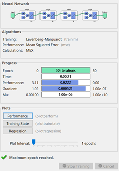
Figure 11 - Letter Recognition newff Function Result
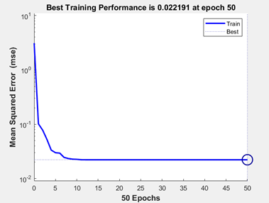
Figure 12 - Letter Recognition Performance
In Figure 12, we can see that around 10th epoch we have always same mean squared error so that we can adjust our epoch number to 10 because it will cost less.
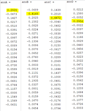
Figure 13 - Letter Recognition Result of Letter A, B, C and D
As you see in Figure 13, we have result for letter A, B, C and D. For example, letter A has highest probability at 1st row. It is reasonable because A is 1st letter. Also, B has highest probability in 2nd row and so on. This result shows that we have correct prediction but not perfect we can still improve our accuracy. Let’s check the martix for result of the all letters.
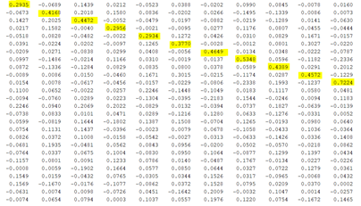

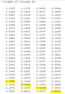
Figure 14 - Letter Recognition Result for All Letters
It is obvious that the diagonal of the “ansALL” matrix has always the highest element for every row so that we prove that we have good neural network training. However, as I told you before we can optimize and get better predictions. Let’s optimize and check our results.
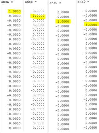
Figure 15 - Letter Recognition Optimized Result of Letter A, B, C and D
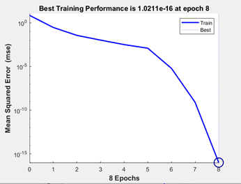
Figure 16 - Letter Recognition Optimized Performance
As you see in Figure 15 and Figure 16 our predictions look perfect. The optimization was made by decreasing the number of the hidden layers. The reason why hidden layers numbers were decreased is hidden layers are useful for more complex problems, they extract some features from inputs such as images. However, for this problem, it is unnecessary to apply a lot of hidden layers. We have used 8 epochs because it reached the best MSE at the 8th epoch.
Now, I want to explain what is Mean Square Error. Mean Squared Error represents the average of the squared difference between the original and predicted values in the data set. It measures the variance of the residuals.
I will add some noise to our data set for the letter recognition and test the change of the mean square error (Figure 17).
%% When there is error
% Error (We make noise here)
pA_err = PA;
pA_err(2:4) = 0.88;
error_A=sim(net,pA_err')
Figure 17 - Letter Recognition with Noise
I added some different values like 0.88 to the input vector just for the letter A. Before adding the noise we had a perfect prediction. Let’s see now how it change.
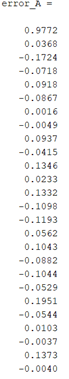
Figure 18 - Noisy Result
As you see in Figure 18, we still have good prediction for letter A but the probability has decreased. This is end of the first project. Now it is time for explaining project 2.
In this project, our aim is to give 5 different images (Figure 19) which are 210x240 pixels to the neural network in the form of binary, train them and finally correctly predict the image after training. Let’s first check our MATLAB code one by one. Firstly 5 different images were added to MATLAB as shown in Figure 20. Also, the size function is used to check the size of the images.

Figure 19 - 210x240 Pixel 5 Images
%% Image Recognition Extended
image1 = imread("image1.jpg"); % Reading image - 1
image2 = imread("image2.jpg"); % Reading image - 2
image3 = imread("image3.jpg"); % Reading image - 3
image4 = imread("image4.jpg"); % Reading image - 4
image5 = imread("image5.jpg"); % Reading image - 5
%% Size Check
size(image1)
size(image2)
size(image3)
size(image4)
size(image5)
Figure 20 - Reading Images on MATLAB
When the size of the images was checked, it was seen that the images have a 210x240x3 matrix which means it is 3 dimensions. We already know that 210x240 is pixel number but what is the meaning of 3? This 3 means that it has three colors (Red, Green, Blue). Therefore, it is better to convert it to gray scale to avoid complexity as shown in Figure 21.
%%  From rgb to gray scale - We want 2 dimensions
image1_gray = rgb2gray(image1);
imshow(image1_gray)
image2_gray = rgb2gray(image2);
imshow(image2_gray)
image3_gray = rgb2gray(image3);
imshow(image3_gray)
image4_gray = rgb2gray(image4);
imshow(image4_gray)
image5_gray = rgb2gray(image5);
imshow(image5_gray)
Figure 21 - Image Recognition from RGB to Gray Scale on MATLAB
As it is known that each image has 210x240 matrixes and there are 5 images. Each pixel is an input for ANN so that we have a huge amount of pixels. If we don’t have a very powerful computer, it will take so long time for each epoch in ANN. Therefore, it is better to decrease the size of each image by imresize function on MATLAB (Figure 22).
%% Let's resize for the ANN
P1=imresize(image1_gray,[20 20]);
P1=P1(:);
P2=imresize(image2_gray,[20 20]);
P2=P2(:);
P3=imresize(image3_gray,[20 20]);
P3=P3(:);
P4=imresize(image4_gray,[20 20]);
P4=P4(:);
P5=imresize(image5_gray,[20 20]);
P5=P5(:);
% PA' -> Tanspose
P = [P1 P2 P3 P4 P5];
Figure 22 - Image Recognition Input Preparation
As you can is in Figure 22, we converted each image into a column vector and put them to the input vector whose defined as P. Besides, our new size is 20x20 matrixes which mean 400 input per image. After that, the target vector, free neural network, and epoch number were prepared as shown in Figure 23. Finally, the network is trained and simulated. Now, let’s discuss the results.
%% Target Vector
T1 = [1 0 0 0 0];
T2 = [0 1 0 0 0];
T3 = [0 0 1 0 0];
T4 = [0 0 0 1 0];
T5 = [0 0 0 0 1];
T = [T1' T2' T3' T4' T5'];
%% NN
range = [zeros(400,1) 255*ones(400,1)];
net = newff(range,[20 5],{'tansig' ,'tansig'});
net.trainParam.epochs = 10;
[net, tr, Y, E] = train(net,P,T);
% net = train(net, P, T, 'useGPU', 'yes'); % for faster train
%% Check Model
ans1 = sim(net,P1);
ans2 = sim(net,P2);
ans3 = sim(net,P3);
ans4 = sim(net,P4);
ans5 = sim(net,P5);
ansALL = sim(net,P);
% YPred = classify(net,imdsValidation);
Figure 23 - Image Recognition Target Vector, NN and Simulation
We have one hidden layer and 10 epochs for the ANN (Figure 24). According to performance (Figure 25), which is the mean squared error method, we have a 0.06 MSE value. This performance can be improved by tuning some hyperparameters such as changing hidden layer numbers or increasing epoch numbers. However, we still have good performance and results as it is seen in Figure 26 because every diagonal element has the highest probability. This means that, for example, the first diagonal element is the probability of prediction of image 1 so that we have a 93.46% chance to predict image 1 which is a very good performance.
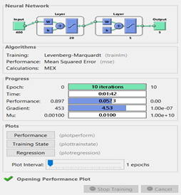
Figure 24 - Image Recognition newff Function Result

Figure 25 - Image Recognition Performance
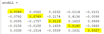
Figure 26 - Image Recognition Final Result
In this repository mainly neural network was investigated. We learned how to create a free neural network, how to add data and train datasets. Also, we simulated our result to see how to correct the estimation we made. After applying basic neural network code, three different projects were explained. The first project aims to predict English Letters correctly. We gave every English Letter to the neural network in the form of binary, train them and finally correctly predict the letters after training. The second project aims to predict 5 different images correctly. We gave 5 different images which are 210x240 pixels to the neural network in the form of binary, train them, and finally correctly predict the image after training.
- [1] Lewis FL. Neural Network Control of Robot Manipulators and Nonlinear Systems. Taylor & Francis; 1999.
- [2] https://purnasaigudikandula.medium.com/a-beginner-intro-to-neural-networks-543267bda3c8
- [3] https://medium.com/dataseries/understanding-the-maths-behind-neural-networks-108a4ad4d4db
- [4] https://towardsdatascience.com/introduction-to-math-behind-neural-networks-e8b60dbbdeba